THE APPLICATION OF THE SECOND KIND CHEBYSHEV WAVELETS FOR SOLVING HIGH-ODER MULTI-POINT BOUNDARY VALUE PROBLEMS

ZHOU Feng-ying,XU Xiao-yong

(School of Science,East China University of Technology,Nanchang 330013,China)

Abstract:In this paper,a numerical algorithm is concerned for solving approximate solutions of high-order multi-point boundary value problems.The second kind Chebyhsev wavelets and operational matrix of integration are used to convert multi-point linear and nonlinear ordinary differential equation to a system of algebraic equations.By comparing with the results of the existing literature,the accuracy and validity of the algorithm for solving the high-order multi-point boundary value problem are explained.The proposed method extends the numerical solution of higher-order multi-point boundary value problems.

Keywords: the second kind Chebyshev wavelets;operational matrix of integration;highorder differential equation;multi-point boundary value problem;collocation method

1 Introduction

The high-order differential equations play a great important role in engineering science,such as mechanics,physics,static electricity,chemical reaction diffusion model, fluid dynamics and so on.They often occur in the form of multi-point boundary value problems(BVPs)for an n-th order ordinary differential equation.For example,an m-point BVP model of a dynamical system with m degrees of freedom.Multi-point boundary value problems arise in a variety of physics area.Many problems in the theory of elastic stability can be handled by the multi-point problems(see[1]).Large size bridges are sometimes contrived with multi-point supports which correspond to a multi-point boundary value condition(see[2]).The existence and multiplicity of solutions of multi-point boundary value problems were studied by many authors,see[3–8]and the references therein.Dehghan and his research group proposed the Adomian decomposition method(ADM)(see[9]),variational iteration method(VIM)(see[10]),homotopy analysis method(HAM)(see[11]),sinc-collocation method(SCM)(see[12])to solve the multi-point BVPs.Shooting method is used to solve multi-point BVPs in[13,14].Reproducing kernel method(RKM)is applied to solve the multi-point BVPs(see[15–19]).By combining the ADM and RKM,Geng and Cui proposed a method for solving nonlinear second order two-point BVP(see[20]).This method is also applied to solve fourth order three-point boundary value problem(see[21]).Di ff erential transform method is used to deal with multi-point BVPs(see[22,23]).Doha developed a method based on shifted Jacobi spectral method for high-order multi-point BVPs(see[24]).In[25],an efficient numerical algorithm based on Haar wavelet is presented to solve a class of linear and nonlinear nonlocal BVPs.To obtain a certain accuracy solution,it needs more collocation points.In[26],the authors applied the augmented block pulse function method for solving a system of arbitrary-order boundary value problem associated with initial conditions or multi-point boundary conditions in separated or non-separated forms.However,some of these methods are reliable and applicable for solving ordinary differential equations,most of them provide the solution only for a particular kind of differential equations or a particular kind of boundary conditions.

In this paper,we consider the multi-point boundary value problems in the following form

with the boundary conditions

i=1,2,···,n,where xj∈ [0,1],j=1,2,···,m.We assume that g has the properties which guarantee the existence and uniqueness of the solution of problem(1.1)under conditions(1.2).The boundary conditions(1.2)can be more general form with linear and nonlinear cases.

Spectral methods play important roles in solving different kinds of differential equations.The main advantage of these methods lies in their accuracy for a given number unknowns.There are three widely used spectral methods,namely,Galerkin,collocation and Tau methods.During the last two decades,wavelets has been paid considerable attention from many scholars and has been applied in wide range of engineering disciplines.Especially,these wavelets constructed from orthogonal polynomials are widely used in seeking numerical solutions of various types of differential equations.Recently,the operational matrices for Legendre wavelet,Chebyshev wavelet and Bernoulli wavelet were extensively used to solve differential equations.

Motivated by the work mentioned above,the main aim of this paper is to find a simple and accurate method based on the second kind Chebyshev wavelets(SCW)for the solution of problem(1.1)under conditions(1.2).Also we want to further extend the applications of the second kind Chebyshev wavelets.Our method consists of reducing the multi-point BVPs to a set of algebraic equations through expanding the highest derivativeμ(n)(x)by the second kind Chebyshev wavelets with unknown coefficients.By solving these coefficients,we get the required approximate solution.In this paper,the application of the second kind Chebyshev wavelets spectral collocation method for finding an approximate solution for multi-point BVPs is investigated.

The rest part of this paper is organized as follows.In Section 2,the second kind Chebyshev wavelets and their properties are introduced.In Section 3,the proposed method is applied to solve high-order multi-point BVPs.In Section 4,we present some numerical examples to show the efficiency and applicability of this method for multi-point BVPs.Finally,a brief conclusion is given in Section 5.

2 The Second Kind Chebyshev Wavelets and Their Properties

The second kind Chebyshev wavelets ψn,m(t)= ψ(k,n,m,t)have four arguments:k can assume any positive integer,n=1,2,3,···,2k?1,m is the degree of the second kind Chebyshev polynomials.They are defined on the interval[0,1)as

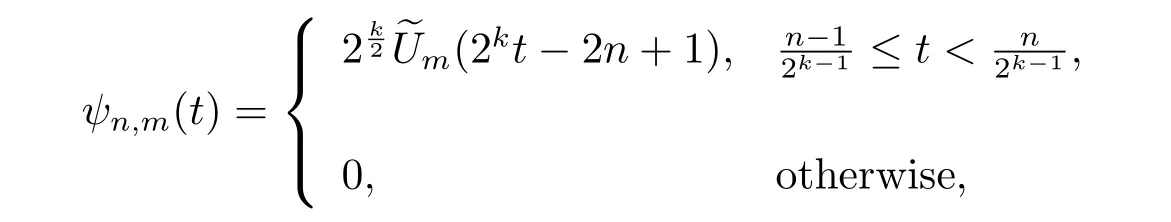
where

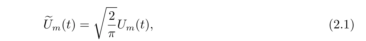
m=0,1,2,···,M ? 1 and M is a fixed positive integer.The coefficient in eq.(2.1)is for orthonormality,here Um(t)are the second kind Chebyshev polynomials of degree m which are orthogonal with respect to the weight function ω(t)=on the interval[?1,1]and satisfy the following recursive formula

Note that when dealing with the second kind Chebyshev wavelets the weight function has to be dilated and translated as ωn(t)= ω(2kt? 2n+1).

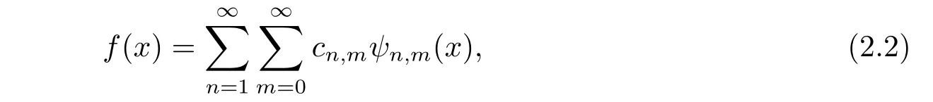
A function f(x)∈L2(R)defined over[0,1)may be expanded by the second kind Chebyshev wavelets as

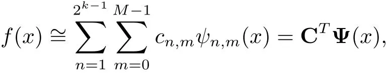
where C and Ψ(x)are 2k?1M × 1 matrices given by

The following theorem gives the convergence and accuracy estimation of the second kind Chebyshev wavelets expansion(see[28]).

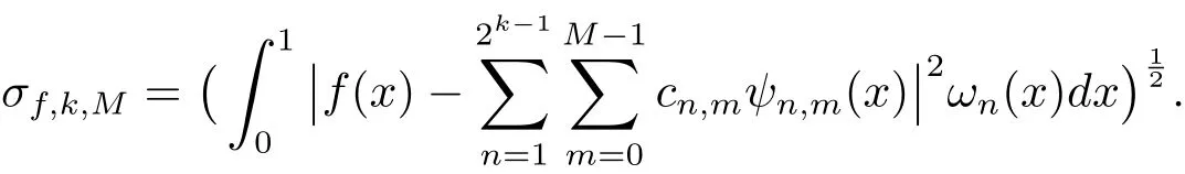
Theorem 2.1 Let f(x)be a second-order derivative square-integrable function defined on[0,1)with bounded second-order derivative,say|f′′(x)|≤ B for some constants B,then

(i)f(x)can be expanded as an in finite sum of the second kind Chebyshev wavelets and the series converges to f(x)uniformly,that is

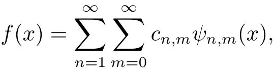
where cn,m= ?f(x),ψn,m(x)?L2ω[0,1).

(ii)

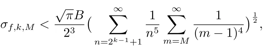
where

The operational matrix of integration of the second kind Chebyshev wavelets with omitted item has been derived in(see[28]),which plays very important role in solving high-order multi-point boundary value problems.For k=3 and M=3,let

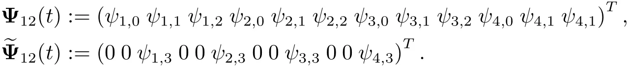
Then we have the following expression

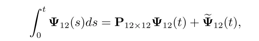
where

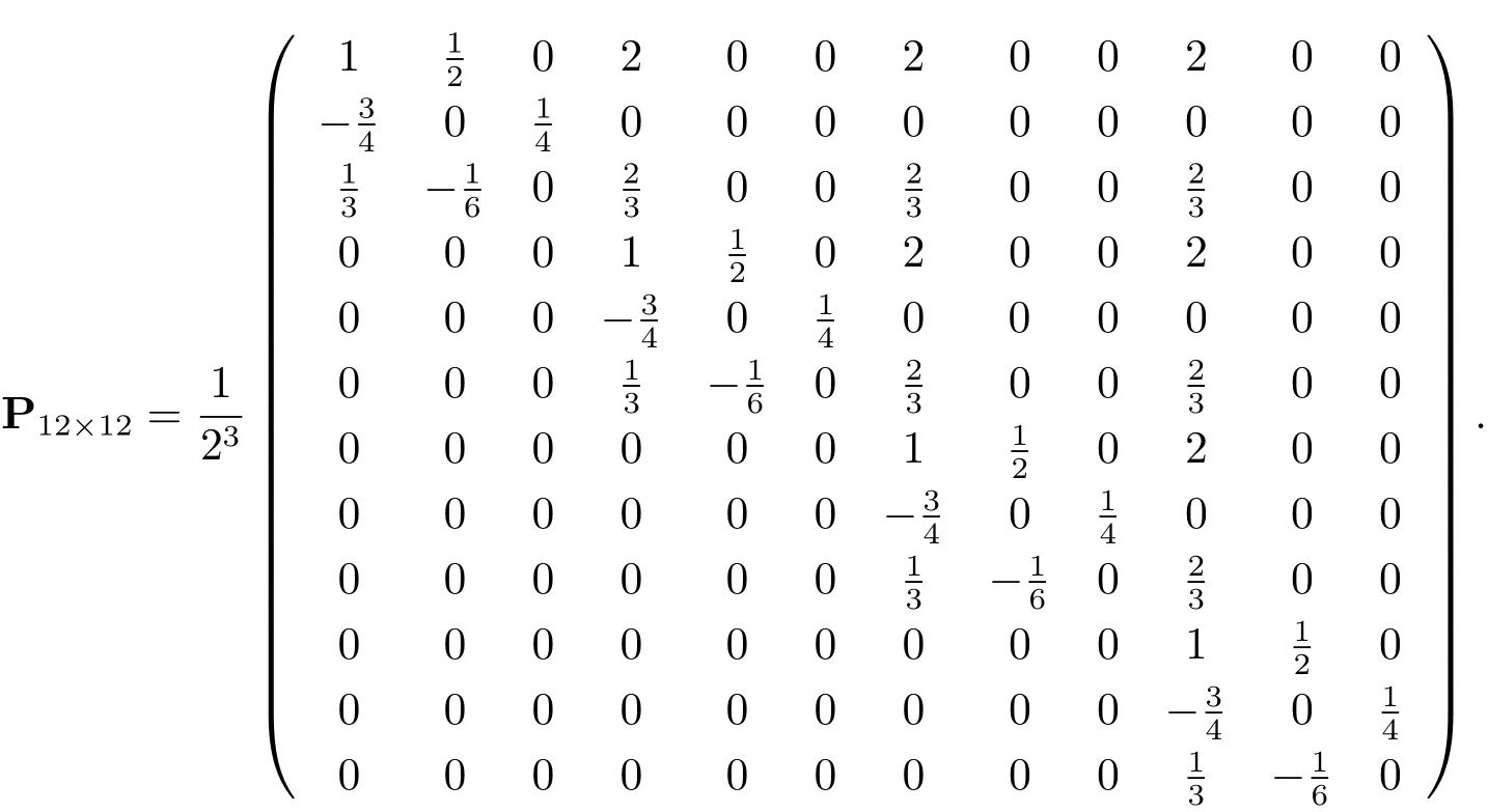
In fact,the matrix P12×12can be written as

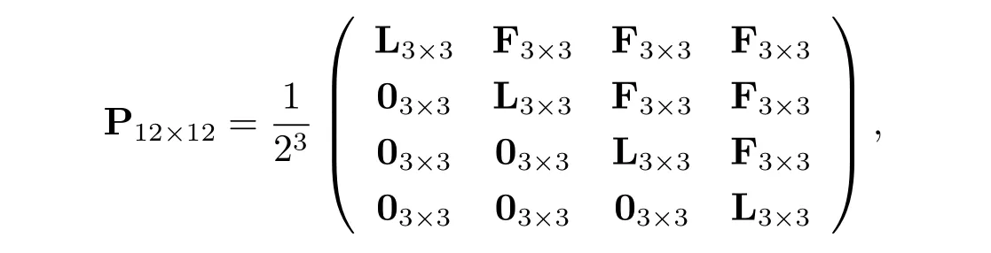
where

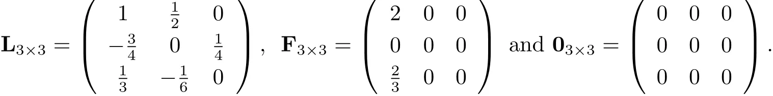
In general,when M≥4,it follows

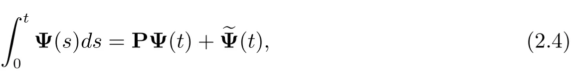
where Ψ(t)is given in(2.3)and P is a 2k?1M × 2k?1M matrix given by

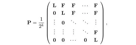
here L and F are M×M matrices given by

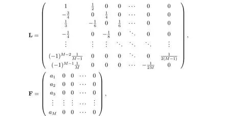
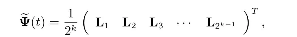
where Liare 1×M matrices given by

3 Description of the Proposed Method

In this section,numerical solution of BVPs with multi-point boundary conditions based on the second kind Chebyshev wavelets is discussed.We assume that the highest derivative in the differential equation is approximated by the second kind Chebyshev wavelets as below

where C is an unknown vector which should be determined and Ψ(x)is the vector defined in(2.3).Before the further description of the proposed method,we introduce the following notations first

Integrating eq.(3.1)and by eq.(2.4),we get

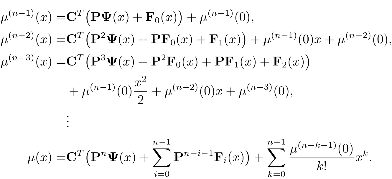
Without loss of generality,we may assume the values ofμ(k)(0),k=0,1,2,···,n ? 1 are unknowns such that

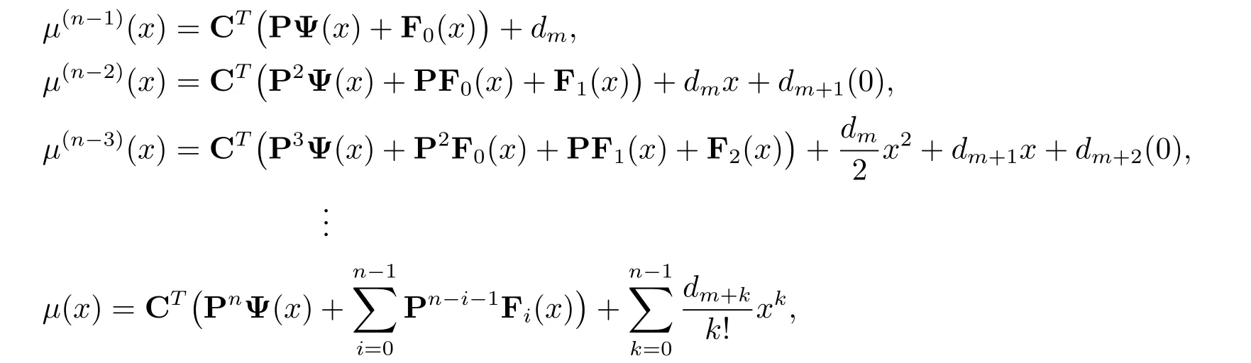
where dm+k= μ(n?k?1)(0),k=0,1,2,···,n?1.In order to calculate unknown vector C in(3.1),the following collocation points are considered

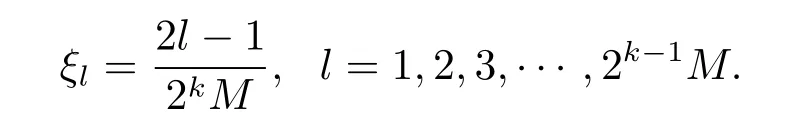
We replace the expression of μ(i)(x),i=0,1,2,···,n,into systems of(1.1)and(1.2),and then substitute the collocation points as follows

and

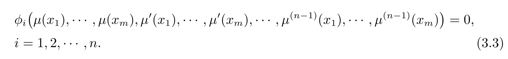
From eqs.(3.2)and(3.3),a system of 2k?1M+n equations and 2k?1M+n coefficients is obtained.Solving this system,we can get the unknown vector C and therefore the functionsμ(i)(x),i=0,1,2,···,n,are identified.Note that we can do a few simple modifications when some ofμ(i)(0),i=0,1,2,···,n ? 1 are given.Particularly ifμ(i)(0),i=0,1,2,···,n ? 1 are all given,the system becomes an initial value problem and there is no need to consider any di,i=m,m+1,···,m+n ? 1.

Remark 1 For linear multi-point BVPs,the coefficients diare expressed by Ψ(x),and unknown vector C.The unknown functionμ(x)and its derivatives are substituted into eq.(3.2)and then collocation method is applied to generate linear system which can be solved using Gauss elimination method.The solution of this system gives us the values of unknown vector C.We can calculate the approximate value of the unknown functionμ(x)at any point using vector C.

Remark 2 For nonlinear case,after substituting Chebyshev wavelet expression ofμ(x)and its derivatives and collocation points into eqs.(3.2)and(3.3),a nonlinear system of 2k?1M+n equations is obtained.This nonlinear system may be solved by using any iterative method for nonlinear system such as Newton’s method,Broyden’s method etc.Solving this system gives us the values of unknown vector C and di,which can be used to find approximate solution in a similar way as discussed for linear case.

Newton’s iterative method for the nonlinear system F(x)=0,where F:? ? Rn→ Rnis defined by xk+1=xk?[F′(xk)]?1F(xk),where F′(xk)is the Jacobian matrix of point xk.

4 Numerical Examples

In this section,we give some numerical examples to demonstrate the efficiency and reliability of the proposed method.We also complete all the numerical computation and reported the absolute error at the selected points in tables and figures.

Example 1 Consider the following second-order four-point nonlinear ordinary differential equation[15,29]

with the boundary conditions

where f(x)=6cosh(x)+sinh(x)(2+x?x2+sinh(x)).The exact solution is given byμ(x)=sinh(x).In Table 1,we list the absolute errors at some different points obtained by the present method with k=3 and M=4,6,8,10.As we see from this table,it is clear that the result obtained by the present method is superior to that obtained by the numerical methods given in[15,29].In Figure 1,we display the logarithmic plot for the maximal absolute errors at selected points with k=3 and M=3 through 10 and the logarithmic plot for absolute errors with different M and different methods.

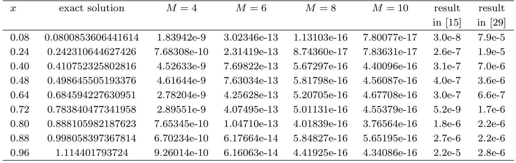
Table 1:Comparison of absolute errors for Example 1 with k=3

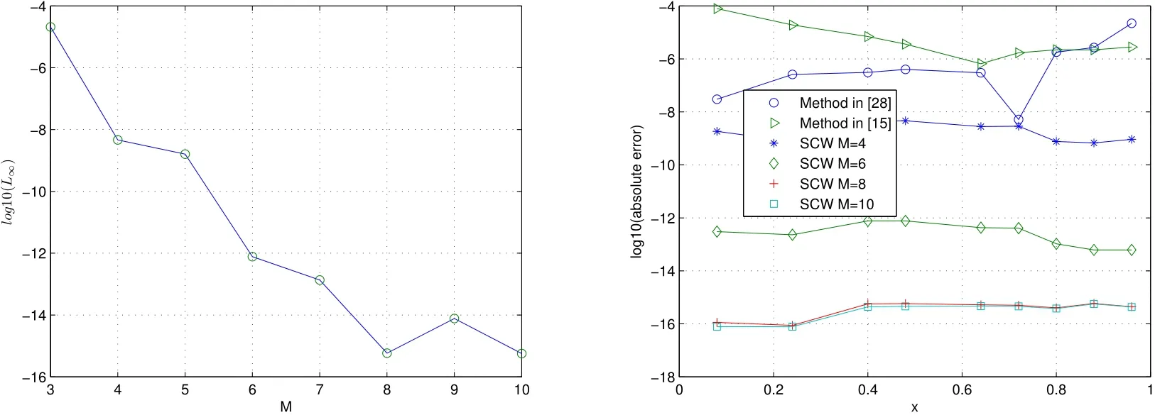
Figure 1:The logarithmic plot for the maximal absolute errors for Example 1(left)and the logarithmic plot for absolute errors for Example 1(right)

Example 2 Consider the following third-order three-point nonlinear boundary value problems(see[13]) μ′′′(x)=e?xμ2(x),0 ≤ x ≤ 1 with the following nonlinear conditions

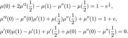
The exact solution isμ(x)=ex.In Table 2,we compare the absolute errors at some different points obtained by the present method and the Newon-Broyden shooting method(NBSM)in[13].In Figure 2,we show the logarithmic plot for the maximal absolute errors at selected points with k=3 and M=3 through 10 and the logarithmic plot for absolute errors with different M and different methods.It is evident from the figure that accuracy of the method increases with the increase of number M.

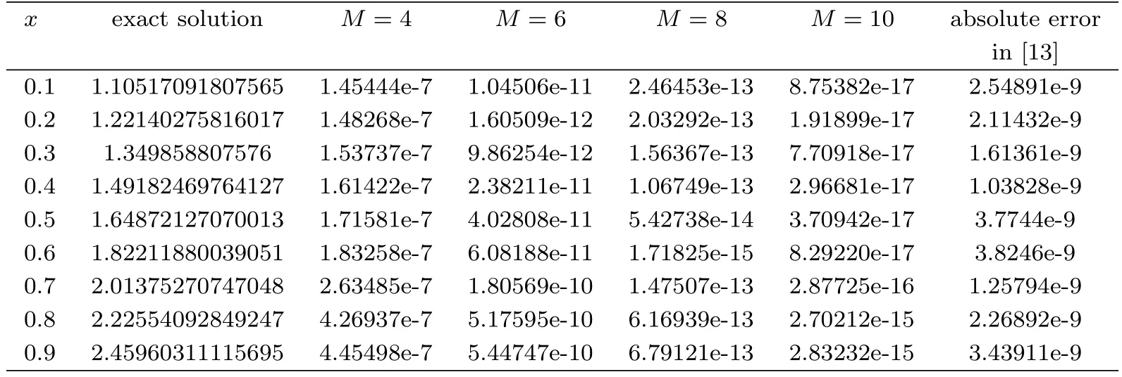
Table 2:Comparison of absolute errors for Example 2 with k=3

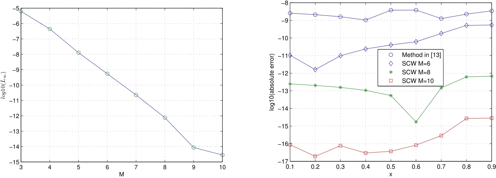
Figure 2:The logarithmic plot for the maximal absolute errors for Example 2(left)and the logarithmic plot for absolute for Example 2 errors(right)

Example 3 Consider the following fourth-order three-point linear boundary value problem[18,22]

with boundary conditions given by

The exact solution isμ(x)=1+sinh(x).In Table 3,we compare the absolute errors at some different points obtained by the present method and reproducing kernel methods in[18]and differential transform method in[22].In Figure 3,we show the maximum absolute errors at selected points with k=3 and M=3 through 10 and the logarithmic plot for absolute errors with different M and different methods.Comparing with the Haar wavelet method in[25],we obtain more accurate solution in the case of the same number of collocation points.When the number of collocation points is 32,our result L∞=5.8987e-11,while in[25]L∞=4.2510e-7.

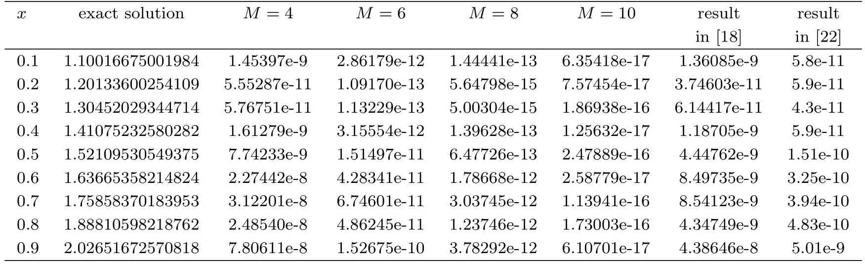
Table 3:Comparison of absolute errors for Example 3 with k=3

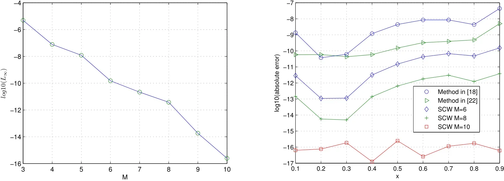
Figure 3:The logarithmic plot for the maximal absolute errors for Example 3(left)and the logarithmic plot for absolute errors for Example 3(right)

Example 4 Consider the following fifth-order four-point boundary value problems[18]

with boundary conditions given by

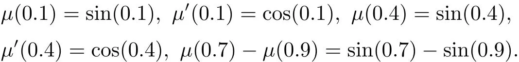
The exact solution isμ(x)=sinx.In Table 4,we compare the absolute errors at some different points obtained by the present method and the reproducing kernel method(RKM)in[18].In Figure 4,we show the maximum absolute errors at selected points with k=3 and M=3 through 10 and the logarithmic plot for absolute errors with different M and different methods.

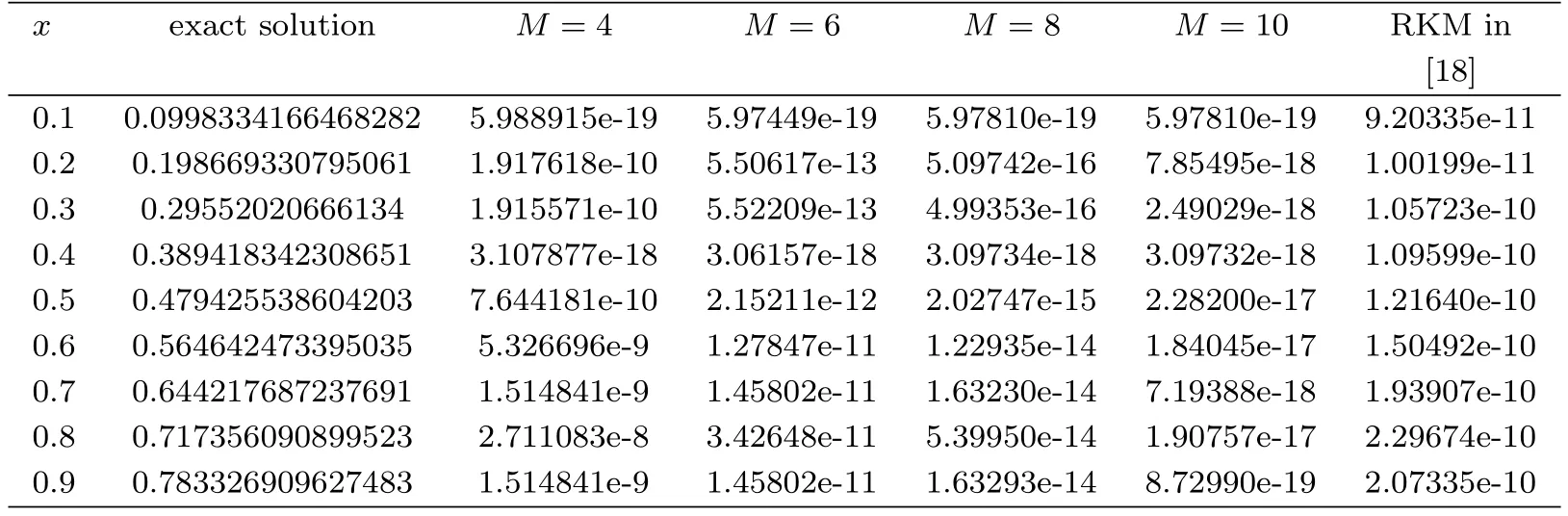
Table 4:Comparison of absolute errors for Example 4 with k=3

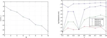
Figure 4:The logarithmic plot for the maximal absolute errors for Example 4(left)and the logarithmic plot for absolute errors for Example 4(right)

Example 5 Consider following seventh-order three-point nonlinear boundary value problems[31]

with boundary conditions given by

The exact solution isμ(x)=(1?x)ex.In Table 5,we compare the absolute errors at some different points obtained by the present method and variational iteration method(VIM)in[31].In Figure 5,we show the maximum absolute errors at selected points with k=3 and M=3 through 10 and the logarithmic plot for absolute errors with different M and different methods.

Remark 3 In the all figures(left side),a logarithmic scale is used for the error-axis.It is obviously that the errors show an exponential decay,since in these semi-log representations one obverse that the error variations are essentially linear versus the polynomial degrees for all the examples.That is the so-called spectral accuracy as expected since the exact solution is smooth.

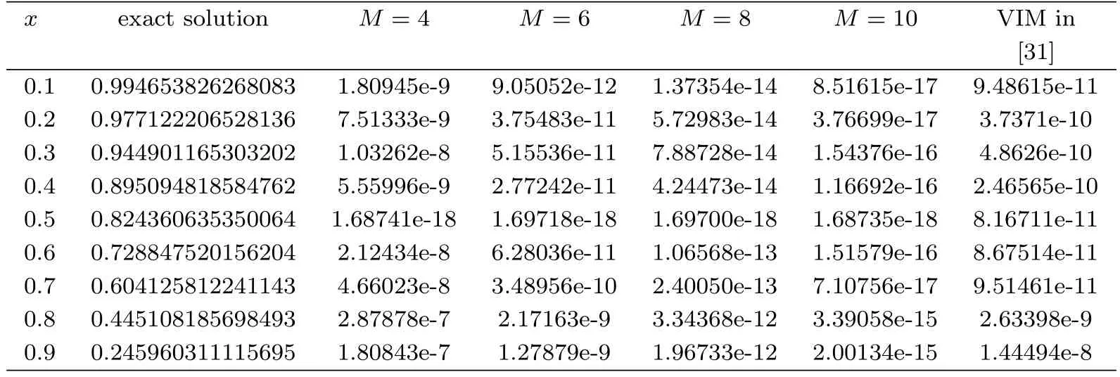
Table 5:Comparison of absolute errors for Example 5 with k=3

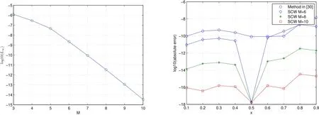
Figure 5:The logarithmic plot for the maximal absolute errors for Example 5(left)and the logarithmic plot for absolute errors for Example 5(right)

5 Conclusion

In this paper,the second kind Chebyshev wavelet collocation is applied to find numerical solutions of high-order multi-point boundary value problems.One of the advantages of the developed algorithm is that it can be applied on both linear and nonlinear problems and performs equally well in both cases.Another advantage is that high accurate approximate solutions can be achieved by using a few number of Chebyshev wavelet basis functions.Illustrative examples are presented to demonstrate the validity and applicability of the algorithm.