Hopf Bifurcation of Cross Diffusion Predator-Prey Model with Herd Behavior and Delay

CHENG Fangyuan(程方圓),ZHANG Tiansi(張天四)

(University of Shanghai for Science and Technology,Shanghai 200093,China)

Abstract: In this paper,we study the Hopf bifurcation of cross diffusion predator-prey model with herd behavior and delay.Taking the death rate β and the delay τ as bifurcation parameters in the model,we discuss the stability of equilibrium point by Routh-Hurwitz conditions and the existence of Hopf bifurcation induced by cross diffusion and delay respectively by analyzing characteristic equation.We get the result that the Hopf bifurcation of the system occurs when β and τ pass through the critical values.Finally,we carry out numerical simulation to verify the correctness of the conclusion.

Key words: Predator-prey model;Hopf bifurcation;Cross diffusion;Delay;Stability

1.Introduction

Biological mathematic is an important branch of modern applied mathematics.More and more predator-prey models are proposed with the development of biology and mathematics.We know that there are many factors that affect population dynamics in predator-prey relationships and functional response can be classified into many different types such as Holing I-IV type,Hassell-Varley type,Beddington-DeAngelis type,Crowley-Martin type,and so on.And the stability of equilibrium and bifurcation are studied.Hale[1]first studied the local bifurcation of delay differential system.He studied the existence of central flow patterns for delay differential system and Hopf bifurcation theorem.Recently,the study of the stability of delayed differential equation and Hopf bifurcation have attracted the attention of many scholars[2?3].They showed that delay can destabilize the positive equilibrium and induce Hopf bifurcation.Some scholars[4?6]combined delay with diffusion,the local stability of the positive equilibrium and delay-induced and diffusive-induced Hopf bifurcation are investigated.In this paper,we add the time delay and diffusion to the predator-prey model with herd behavior to study its Hopf bifurcation.

In [7],Ajraldi,Pittavino and Venturino investigated the classical two population system and showed that under suitable assumptions in some instances it may lead to unexpected behavior.

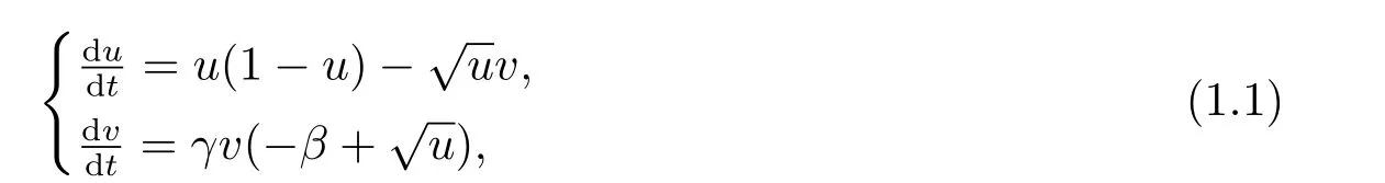
hereu(t) andv(t) stand for the prey and predator densities,respectively,at timet.βγis the death rate of predator in the absence of prey.γis the conversion or consumption rate of prey to predator.

Recently TANG and SONG[8]have investigated the cross-diffusion induced spatiotemporal patterns in a predator-prey model with herd behavior.They gave the conditions for cross-diffusion induced instability and derived amplitude equations for the excited modes.

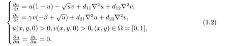
whered11>0 andd22>0 are diffusion coefficients for prey and predator respectively.The coefficientsd12andd21are called cross-diffusion coefficients describing the population fluxes of prey and predators resulting from the presence of the other species,respectively.

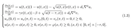
In 2015,TANG and SONG[6]studied the stability,Hopf bifurcations and spatial patters in delayed diffusive predator-prey model with herd behavior.By choosing the appropriate parameter,they got the result that Hopf bifurcations can be induced by diffusion and delay respectively.And they obtained the formula determining the properties of the Hopf bifurcation in.

As known,biology species often do not response to the variation of the environment instantaneously,instead,they generally response to the variations in the past.Sometimes,the predator does not consume the prey instantaneous,there are some constant time to consume for predator.Due to this point,we combine the factor of cross-diffusion in the system (1.2)with the facter of delay in the system (1.3),then get the following system (1.4):

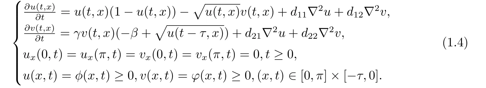
With the same aim,we discuss the stability of positive equilibrium and the corresponding Hopf bifurcation.

As the beginning,we give an assumption:

which indicates that the flow of the respective densities in the spatial domain depend more strongly on their own density than on the others[9],whereτis the delay item.

2.Stability of Positive Equilibrium

This section is to discuss the stability of positive equilibrium of the system (1.4).It is clear that the system has two boundary equilibriaE1(0,0),E2(1,0) and a unique positive equilibriumE3(u?,v?) if 0<β <1,whereu?=β2,v?=β(1?β2).Since we are looking for the stability of the positive equilibrium point,we omit the boundary equilibrium points here.

Suppose that there is neither diffusion nor delay,then the system (1.4) can be reduced into the system (1.1),which has the Jacobian

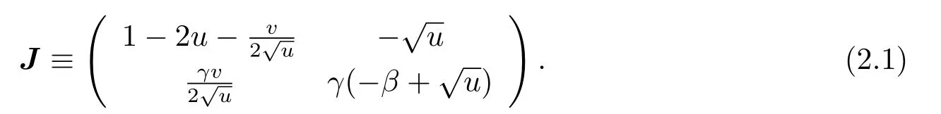
By the Routh-Hurwitz conditions for interior equilibrium,we have

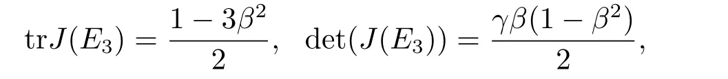
From the above discussion and those in [7],we can get the following lemma.

Lemma 2.1Forthe system (1.1) possesses a limit cycle and has an unstable positive equilibriumE3(u?,v?);Forthe system (1.1) has a globally asymptotically stable positive equilibriumE3(u?,v?);While forthe system (1.1)undergoes a Hopf bifurcation nearE3(u?,v?).

But the above is the fraction of the system(1.1)without delay and diffusion.So to make the question more suitable,we consider the delay and the diffusion in the system (1.4).For the convenience of discussion,we useu(t)foru(t,x),v(t)forv(t,x)andu(t?τ)foru(t?τ,x).Let

The linearization of system (1.4) atE3(u?,v?) is

whereand

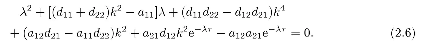
The characteristic equation of (2.3) is：

whereIis the 2×2 identity matrix andThen the sequence of quadratic transcendental equations at the positive equilibriumE3(u?,v?)is

Setτ= 0.(2.6) can be written as the following sequence of quadratic polynomial equations:

where

3.Hopf Bifurcation Induced by Diffusion

In this section,takingτ= 0,we consider the Hopf bifurcation induced by diffusion in(2.7) fork ≥1.According to the condition of Hopf bifurcation,we haveTk= 0,Dk >0.From (2.8),Tk(β)=0 yields

Clearly (2.4) gives the following results

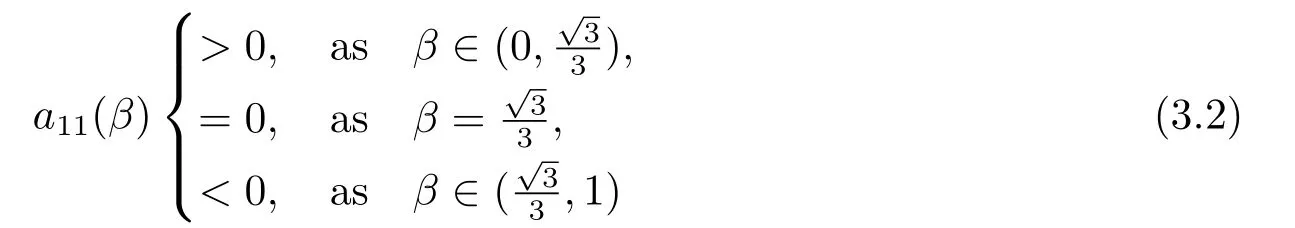
andForthena11(β)<0,Tk=(d11+d22)k2?a11(β).SoTkmust be greater than zero.It does not meet the conditions for Hopf bifurcation.Therefore,the potential bifurcation points of the system (1.4) belong to

Next,we look for the exact value ofβ.Solving (3.1),we have

For this bifurcation point 0<βk <1,we have the following results.

Lemma 3.1Assume 0<βk <1.Then the bifurcation points are finite,that is,there is a non-negative integerand N1∈N0,such thatβkare(resp.not)bifurcating points if 0≤k ≤N1(resp.k >N1).

ProofWhen 0≤β ≤1,Maxa11(β) =a11(0),that is,a11(0)<(d11+d22)k2whenkis big enough.So there isTk(β)<0.Then (2.6) does not exist any purely imaginary roots.MakingTk(β) = 0,we have a unique solutionand there is no solutions asThis competes the proof.

Lemma 3.2Assume 0<βk <1.Then for any 0≤k ≤N1,there is 0<βN1<··· <βk <···β0<1.

ProofFrom (3.3),we can easily see that the value ofβincreases with the decrease ofk.This competes the proof.

To generate bifurcation,Tk(βk)= 0,Dk(βk)>0 as 0≤k ≤N1,andTj(βk)≠0 for anyj≠k.In order to meet the above conditions,we make the second hypothesis:(H2)

Under hypothetical conditions,we verify the transverse condition.

Lemma 3.3Assume(H1)and(H2)hold.Then for any 0<β <1,we have Re(λ′(β))<0.

ProofSuppose that the root of (2.7) has the formλ(β) =α(β)+ib(β),whereα(β),b(β)∈R.Since the real part of eigenvalueλisRefor any 0<β <1.This competes the proof.

From Lemmas 3.1-3.3,a statement can be given as follows.

Theorem 3.1Assume(H1)and(H2)hold.When 0<β <1,there are N1+1 bifurcating pointsβksatisfying 0<βN1<···<βk <···β0<1,such that the system (1.4) undergoes a Hopf bifurcation atβk.Moreover,

1)E3(u?,v?) is unstable when

2)E3(u?,v?) is locally asymptotically stable when

3)The periodic solutions bifurcating fromare spatially homogeneous,the periodic solutions bifurcating fromβ=βkare spatially non-homogeneous.

4.Hopf Bifurcation Induced by Delay

Now we discuss the bifurcation induced by delay.Keepstill hold.Whenτ=0,we always assume that the positive equilibriumE3(u?,v?)of the system(1.4)is locally asymptotically stable.

Assume iωis a root of the characteristic (2.5),then we have

Separating the real and imaginary parts of (4.1) leads to

We know sin2ωτ+cos2ωτ=1,so we can get the following equations:

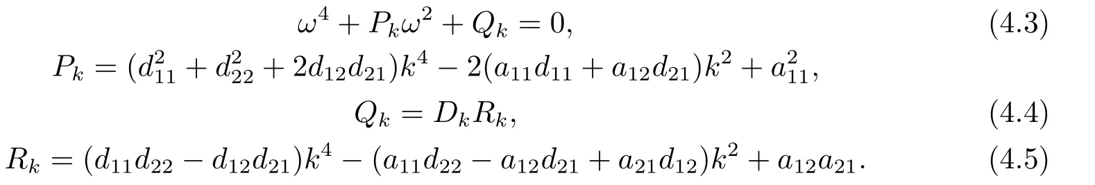
Next we discuss the sign ofPkandQkto determine the value ofω.This is an important step in proving the existence of Hopf bifurcation of the system.

From(4.4),ifanda12=?β <0,we can getPk >0.If(H1)and (H2) hold,thenDk >0 is always true.So the sign ofQkis determined byRk.Notice thatRkis a quadratic polynomial with respect tok2andAccording to (4.5) we can conclude that there exists N2∈N0,such that

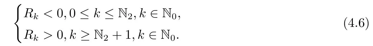
Then forω4+Pkω2+Qk=0,there are

and ?=P2k ?4Qk >0 for eachk ∈{0,1,2···N2}.Therefor (4.3) has the only one positive real rootωk,where

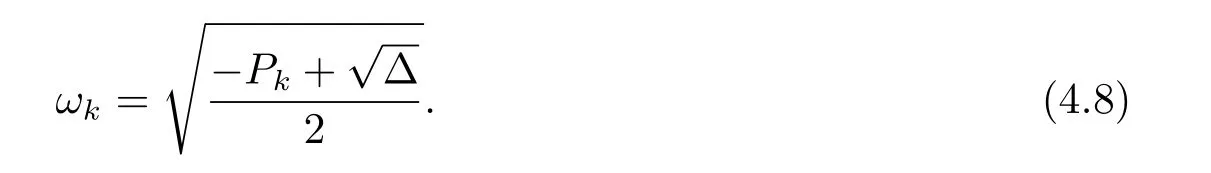
Whenk ≥N2+ 1 andk ∈N0,ω2must be negative if (4.3) is valid,which leads to the nonexistence of real roots of (4.3).

According to the above discussion,we can get the following results:

Lemma 4.1Whenfor allk ∈N0,and N2andωkare defined by (4.6) and(4.8),respectively.(2.5) has a pair of purely imaginary roots±iωkfor eachk ∈{0,1···N2}and has no purely imaginary roots fork ≥N2+1.

From (4.2),fork ∈{0,1,···N2},we can obtain

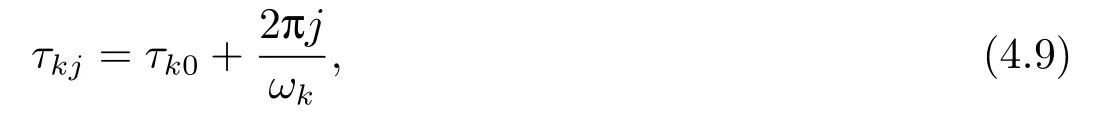
and

Clearly,

Letλ(τ)=α(τ)+iβ(τ)be the roots of(2.6)nearτ=τkjsatisfyingα(τkj)=0,βkj=ωk.Then we have the following transverse condition.

Lemma 4.2Fork ∈{0,1,2···N0}and

ProofDifferentiating two sides of (2.6) onτ,we get,

By (2.6),

Then,

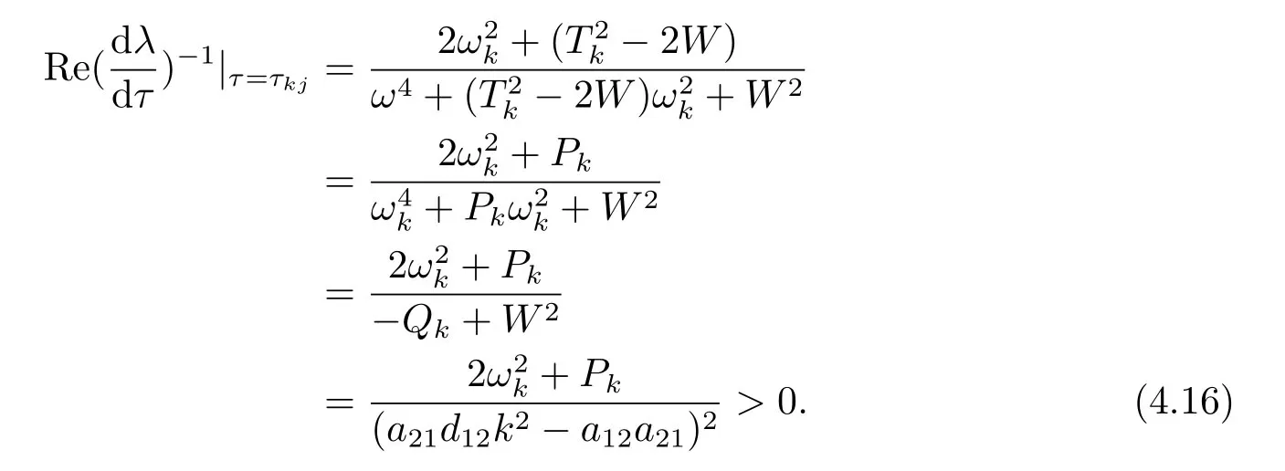
This completes the proof.

From Lemmas 4.1-4.2 and combining with the qualitative theory of partial functional differential equations[10],we come to the following results.

Theorem 4.1Assume (H1) and (H2) hold and for eachk ∈N0,Tk >0,Dk >0 are valid,τ00is defined by (4.9).

1) Whenτ ∈[0,τ00],the system (1.4) has an asymptotically stable positive equilibriumE3(u?,v?);Whenτ ∈(τ00,+∞),(1.4) has an unstable positive equilibriumE3(u?,v?).

2) Whenτ=τ00,the system (1.4) undergoes Hopf bifurcation near the positive equilibriumE3(u?,v?) fork ∈{0,1,···N2}andj ∈N0.Moreover,ifk=0,the bifurcation periodic solutions are all spatially homogeneous.Otherwise,these bifurcation periodic solutions are spatially inhomogeneous.

5.Numerical Simulations

In this section,we present numerical simulations to verify the above conclusion.Fig.5.1 and Fig.5.2 represent quantitative change of predator and prey with fixed the value of delayτand take death rateβas variable.Fig.5.3 and Fig.5.4 represent quantitative change of predator and prey with fixed the value of death rateβand take delayτas variable.In the first case,whenτ= 0,we taked11= 1,d12= 1,d21= 1,d22= 3,γ= 1.Makethencan be calculated by (2.4).Takeand recalculateFrom Fig.5.1,we can see that the curve vibrate constantly.The curves in Fig.5.2 tend to be stable.These phenomenon correspond to the conclusion of Theorem 3.1.is locally asymptotically stable whenAsβpasses through the critical valuethe equilibriumE3(u?,v?)loses its stability and becomes unstable and the periodic solutions bifurcate from

In Case 2,supposeτ≠ 0.Keepd11= 1,d12= 1,d21= 1,d22= 3,γ= 1,β=,then we getτ00≈0.922.Takeτ= 0.01<τ00,and the curves in Fig.5.3 tend to be stable.Takeτ=1>τ00,and the curves in Fig.5.4 become unstable and vibrate larger and larger.These phenomenon correspond to the conclusion of Theorem 4.1.Whenτ ∈[0,τ00],the system(1.4)has an asymptotically stable positive equilibriumE3(u?,v?).Asτpasses through the critical valueτ00,the equilibriumE3(u?,v?) loses its stability and becomes unstable.

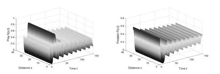
Fig.5.1 The system(1.4) has an unstable positive equilibrium for d11 = 1, d12 = 1, d21 = 1,d22 =3, τ =0, γ =1, β =and the initial conditions (u0,v0)=(u?+0.2175,v?+0.2175).

Acknowledgments:

In this paper,a predator-prey model with time delay and cross-diffusion is established.We study the stability of positive equilibrium point and the existence of Hopf bifurcations with different parameter value.The periodic solutions bifurcating fromβ=are spatially homogeneous,the periodic solutions bifurcating whenβacross through the critical valuesβ1=are spatially non-homogeneous.Meanwhile,the system (1.4) undergoes Hopf bifurcation near the positive equilibrium (u?,v?) atτ=τ00≈0.922.And the bifurcation periodic solutions are spatially homogeneous whenτacross through the critical valueτ=τ00≈0.922.

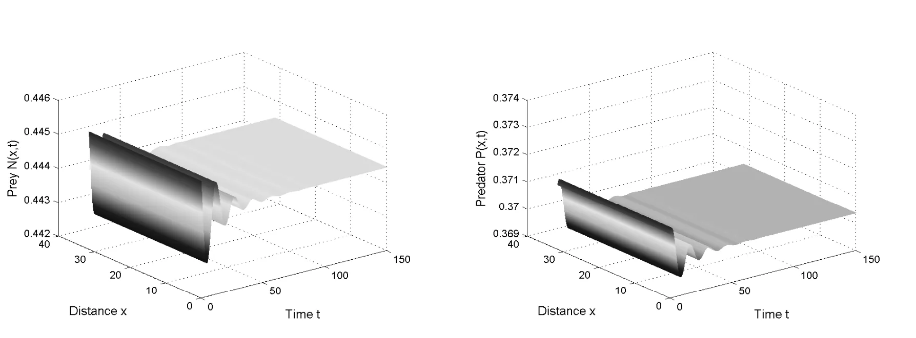
Fig.5.2 The system(1.4) has a stable positive equilibrium for d11 =1, d12 =1, d21 =1, d22 =3,τ =0, γ =1, β = and the initial conditions (u0,v0)=(u?+0.001,v?+0.001).

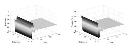
Fig.5.3 The system(1.4) has a stable positive equilibrium for d11 =1, d12 =1, d21 =1, d22 =3,τ =0.1<τ00, γ =1, β =and the initial conditions (u0,v0)=(u?+0.2175,v?+0.2175).

Fig.5.4 The system(1.4) has an unstable positive equilibrium for d11 = 1, d12 = 1, d21 = 1,d22 =3, τ =1>τ00, γ =1, β =and the initial conditions (u0,v0)=(u?+0.001,v?+0.001).

The bifurcation periodic solution are spatially inhomogeneous whenτacross through the critical valueτ= 1>τ00≈0.922.At last,by the numerical simulations,we verified the correctness of the theory and the feasibility of the method.We hope that our work could be instructive to study the population.