OPTIMAL DIVIDENDS WITH EXPONENTIAL AND LINEAR PENALTY PAYMENTS IN A DUAL MODEL

WANG Xiao-fan,MA Shi-xia,LI Tong

(School of Sciences,Hebei University of Technology,Tianjin 300401,China)

Abstract:In this paper,we consider the optimal dividend problem with penalty payments in a dual model.We assume that the company doesn’t go bankrupt when the surplus becomes negative,but penalty payments occur,and the penalty amounts are dependent on the level of the surplus.By using the stochastic optimal control approach and dynamic programming principles,we obtain the HJB equation and verification theorem for the optimal problem.Finally,when the profits follow an exponential distribution,we obtain the optimal dividend strategies and explicit solutions for exponential and linear penalty payments,respectively.

Keywords:dual risk model;dividends;penalty payments;HJB equation

1 Introduction

Recently,many papers were published on the dual risk model.The model is suitable for describing companies whose capital reserves involve a constant flow of expenses and occasional profits,such as petroleum,pharmaceutical or commission-based businesses.In actuarial mathematics,the risk of a company is traditionally measured by the probability of ruin,where the time of ruin is defined as the first time when the surplus becomes negative.Classical ruin probability results for the dual model can be found in Grandell[1],Dong and Wang[2],and Zhu and Yang[3].

Another measure considers the expected discounted dividend payments which are paid to the shareholders until ruin.The dividend problem in the dual model was first introduced by Avanzi et al.[4],and the optional dividend strategy in the dual model was a constant barrier strategy.From then,many researchers studied the dual model under different dividend strategies.See Avanzi and Gerber[5],Gerber and Smith[6],Ng[7]and so on.However,the disadvantage of the dividend approach is that,under the optimal strategy,ruin occurs almost surely.Therefore,the idea of capital injections rises.Whenever the surplus becomes negative,the shareholders have to inject capital in order to avoid ruin.See,for example,Yao et al.[8,9],Avanzi et al.[10]and so on.

All of the approaches above have one thing in common:if the surplus becomes negative,the company either has to inject capital or ruin occurs.However,in practice,it can be observed that some companies continue doing business although they had large losses for a long period.The regulator often intervenes in order to avoid that a company goes out of business.Therefore,it is more realistic to allow negative surplus.In the context of negative surplus,Vierkotter and Schmidli[11]considered optimal dividend problem with penalty payments in a diffusion model.Vierkotter and Schmidli assumed that insurer is not ruined when the surplus becomes negative,but penalty payments occur,depending on the level of the surplus.

Motivated by Vierkotter and Schmidli[11],we consider the optimal dividend problem with penalty payments for a dual model.Similarly,we assume that bankruptcy does not occur,but whenever the surplus is negative,penalty payments occur.These payments reflect all costs which are necessary to prevent bankruptcy.For example,penalty payments can occur if the company needs to borrow money,generate additional equity or additional administrative measures have to be taken.These costs may also be extended to positive surplus to penalise small surplus.The penalty payments are rather technical in order to avoid that the surplus becomes small or even negative.Different from Vierkotter and Schmidli[11],we assume that the dividend payments have transaction costs.

The rest of this paper is organized as follows.In Section 2,the model is described and basic concepts are introduced.In Section 3,the HJB equation and verification theorem for the optimization problem are provided.In Section 4,we explicitly derive the optimal value functions and corresponding optimal strategies for exponential and linear penalty payments when the profits follow an exponential distribution.

2 The Model

Let(?,F,{Ft}t≥0,P)be a filtered probability space on which all stochastic processes and random variables introduced in the following are defined.The company’s uncontrolled surplus process R={Rt}t≥0is the dual model,which is described as

where x≥0 is the initial surplus level;c>0 can be viewed as the rate of expenses;is a compound Poisson process representing the total income amount up to time t,in which N(t)is a Poisson process with a gain arrival intensity λ,and the sequence of gain amounts{Yi}i≥1are independent and identically distributed(i.i.d.)positive random variables with mean m1and a continuously differentiable distribution function F(y).In addition,since E(Rt?x)=t(λm1?c),we assume that the net profit condition,λm1?c>0,is valid.

The manager of the company can control over the dividend payments and the controlled surplus of the company evolves according to

where Dtis the cumulative amount of dividend paid out up to time t.The strategy D={Dt}t≥0is said to be admissible if D is predictable and non-decreasing cádlág processes with D0=0.The set of all admissible strategies is denoted by D.We assume that dividends are paid according to a barrier strategy.Such a strategy has a parameter b>0,the level of the barrier.Whenever the surplus exceeds the barrier,the excess is paid out immediately as a dividend.This means that

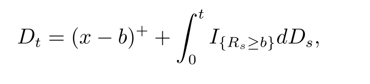
where IArepresents the indiction function of event A.

The value function of a strategy D is defined by

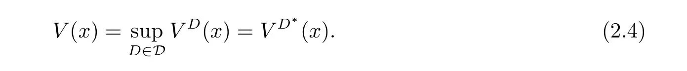
where δ>0 denotes the discount rate,0< η ≤ 1 represents the net proportional of leakages from the surplus received by shareholders after transaction costs are paid.The penalty function φ is continuous,decreasing,and convex a function,satisfying φ(x)→ 0 as x → ∞.The manager’s objective is to find the optimal strategy D?∈ D such that

We have to assume

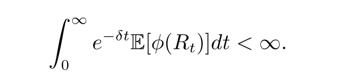
Otherwise,the value function would be minus infinity.Moreover,we assume that

for x

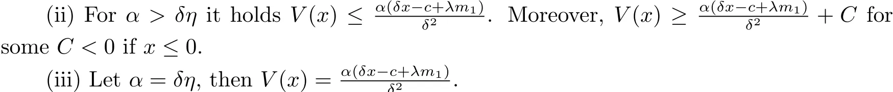
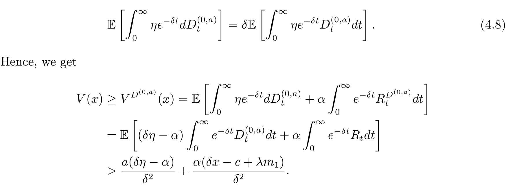
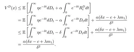
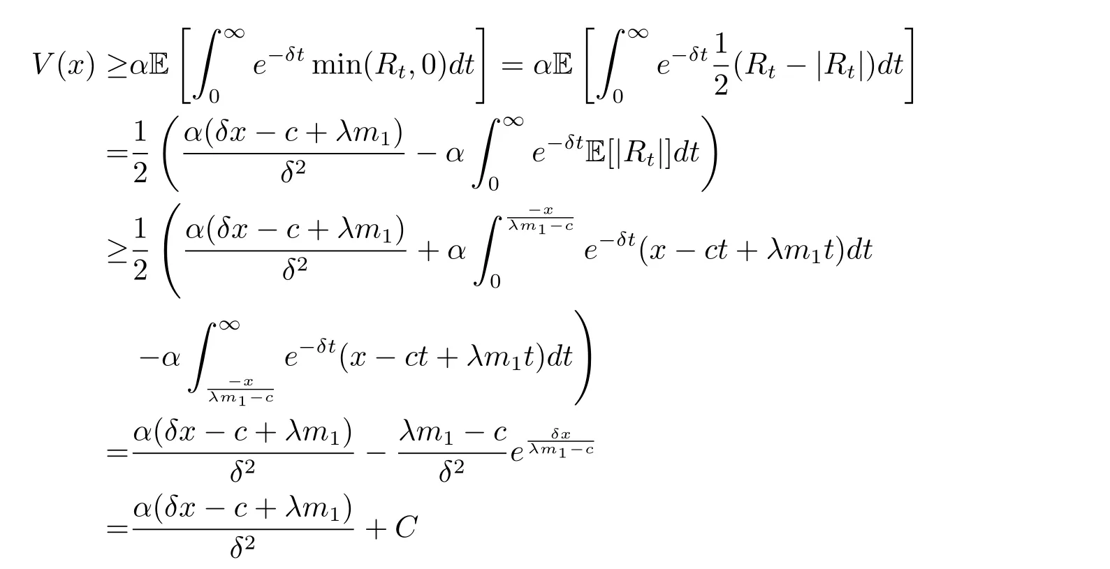
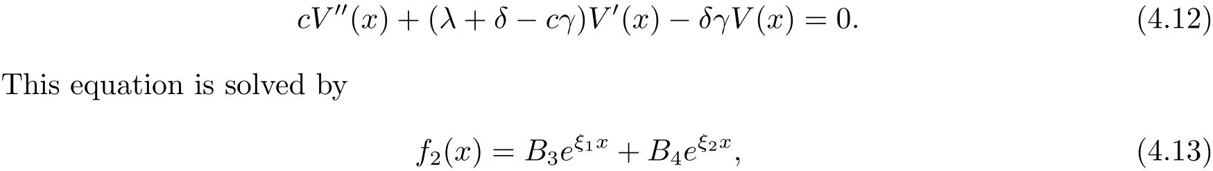
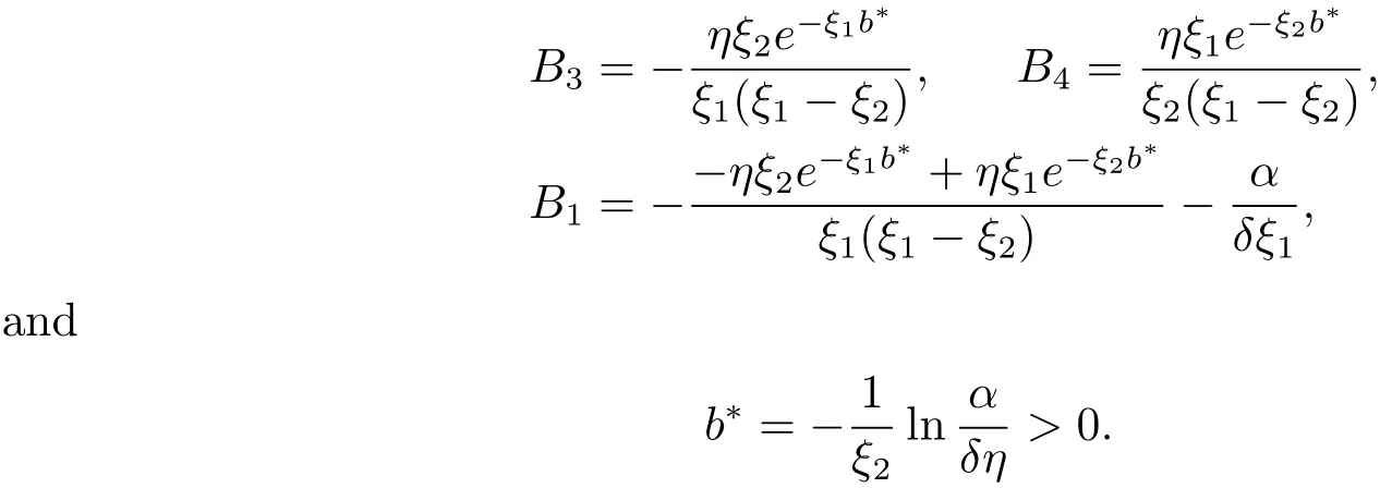
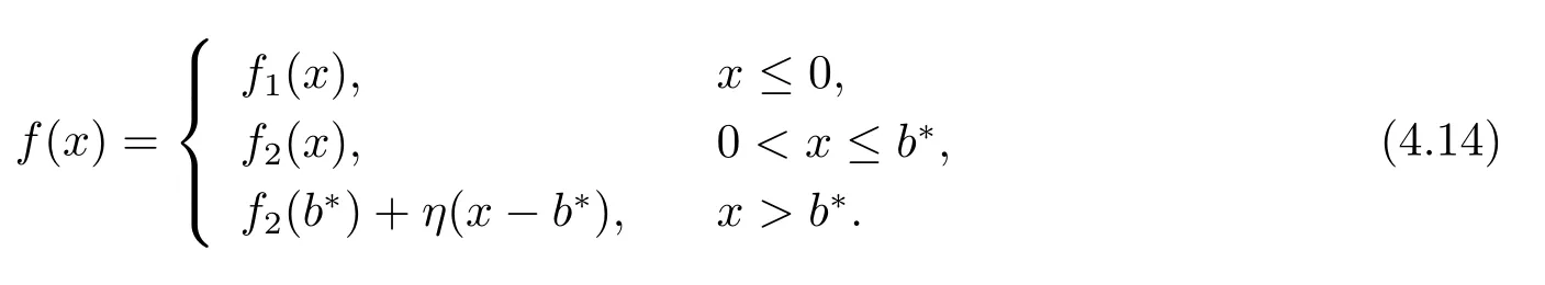
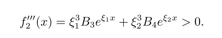
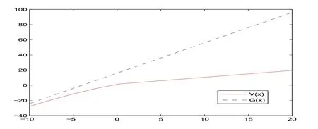
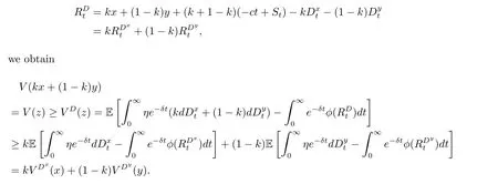
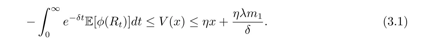
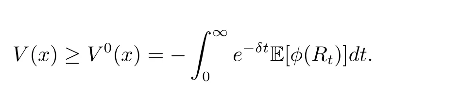
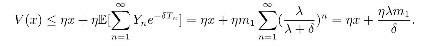
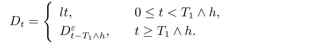
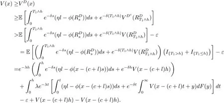
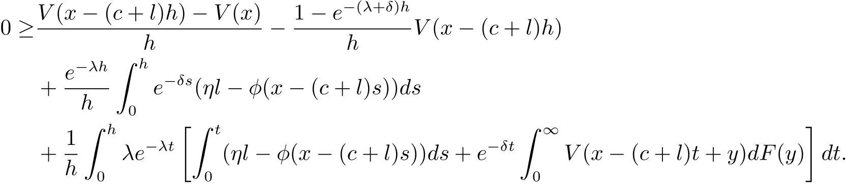
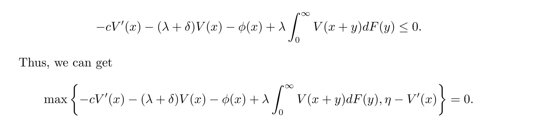
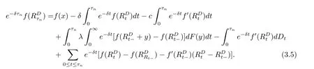
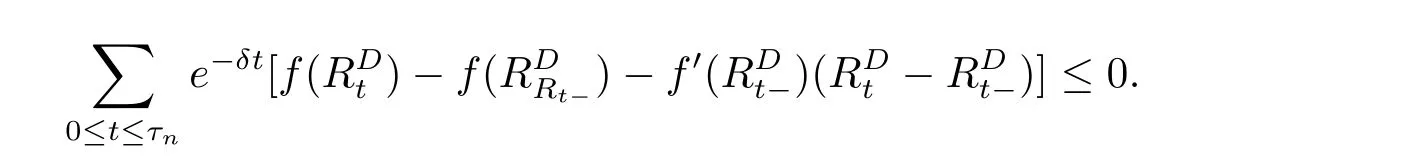
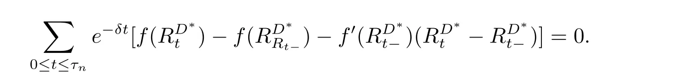
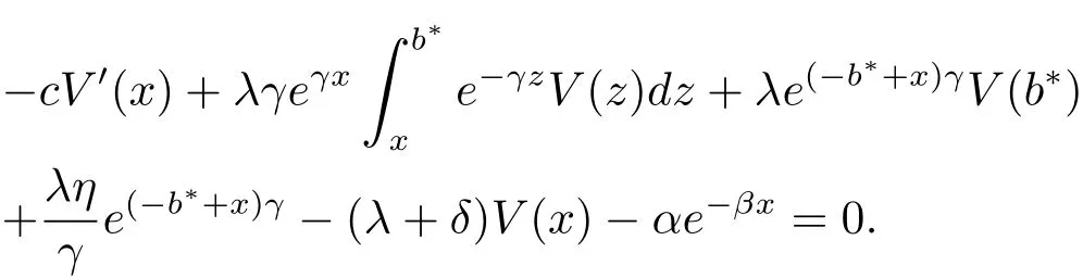
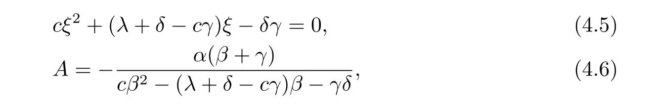
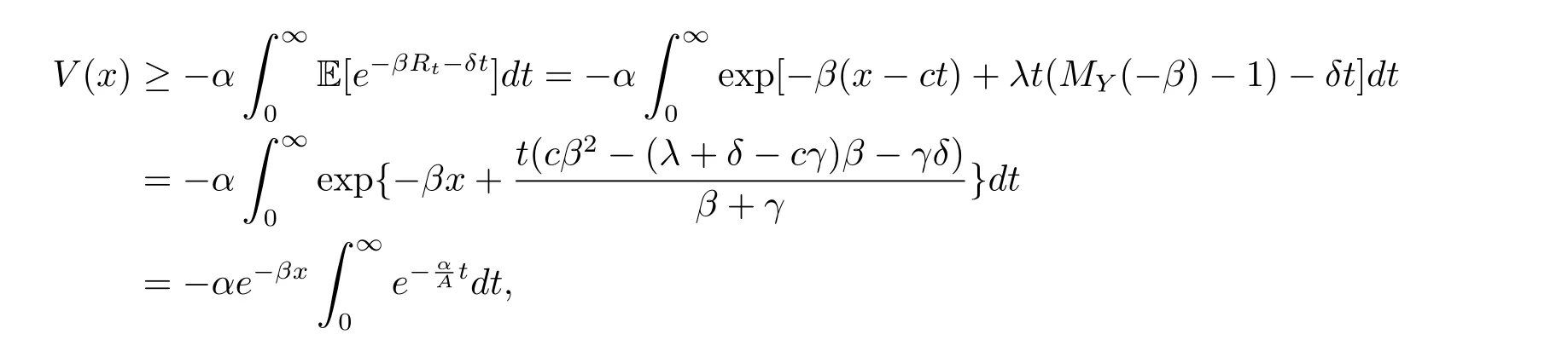
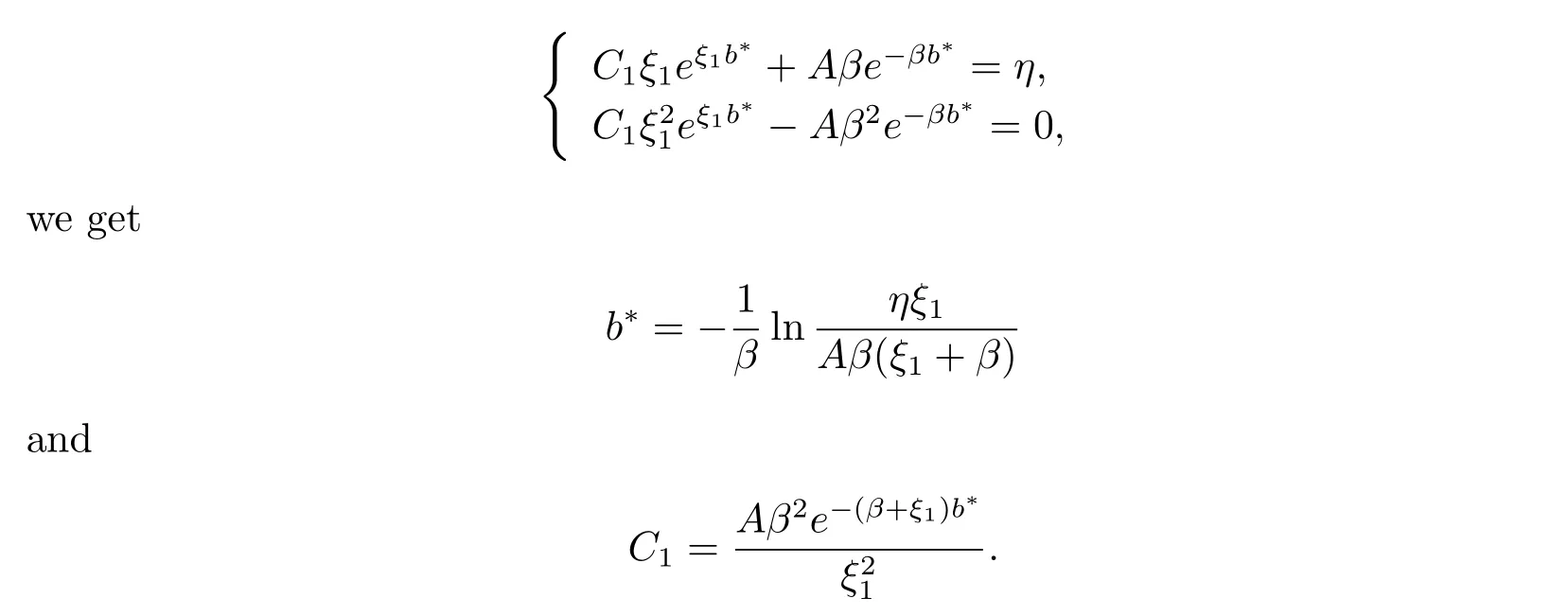
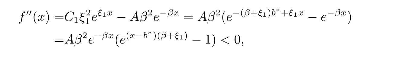
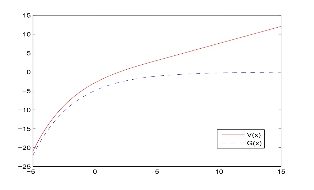
3 The HJB Equation and the Verification Theorem

First,we verify some basic properties of the value function that will help us to prove the following HJB equation.

Lemma 3.1 The function V(x)is concave.

Proof Similarly to Vierkotter and Schmidli[11],let x,y∈R and z=kx+(1?k)y,where k∈(0,1).Applying the strategies Dxand Dyfor initial capital x and y,respectively,we define Dt=k+(1?k)for the initial capital z.Since?φ is concave and

Taking the supremum over all strategies Dxand Dy,we get

This completes the proof.

Remark 3.1 The concavity implies that V is differentiable from the left and from the right and V0(x?)≥ V0(x+)≥ V0(y?)≥ V0(y+)for x

Lemma 3.2 V(x)is increasing with V(y)?V(x)≥η(y?x)for x≤y and

Proof Consider a strategy D with VD(x)≥ V(x)?ε for an ε>0.For y ≥ x,we define a new strategy as follows:y?x is paid immediately as dividend and then the strategy D with initial capital x is followed.Then for any ε>0,it holds that

Since ε is arbitrary,we get V(y)≥ V(x)+ η(y ? x).Hence V is increasing.

Let V0be the value of the strategy where no dividends are paid.Then,Fubini’s theorem implies

On the other hand,consider another extreme case:there is no operating cost(i.e.,c=0),all initial surplus x and profits are paid out immediately as dividends.The company can run smoothly due to no operating costs,there is no penalty payments occur.We find,using the fact that the n-th jump time Tnis Gamma Γ(λ,n)distributed,the upper bound

The proof is completed.

Theorem 3.1 The function V(x)fulfils the Hamilton-Jacobi-Bellman(HJB)equation

where operator A is the infinitesimal generator given by

Proof Let h ≥ 0 and l≥ 0.Consider the strategy Dε,such that VDε(x0)>V(x0)? ε for x0∈ (?∞,x+(c+l)h]and ε>0.Then,we define the strategy

For this strategy,we obtain

Since ε is arbitrary we can let it tend to zero.Then,rearranging the terms and dividing by h implies

Let h→0,we get

Since l is arbitrary,we obtain

If V0(x)< η,then(3.4)would be positive for l large enough.Hence,we can get V0(x)≥ η.In addition,when l=0,we obtain

This completes the proof.

Theorem 3.2 Assume that f is an increasing,concave and twice continuously differentiable solution to(3.2),then f(x)≥ V(x).Moreover,if there exists b?∈ R+such that

(i)(A ? δ)f(x)? φ(x)=0,f0(x)≥ η,?x ≤ b?;

(ii)(A ? δ)f(x)? φ(x)<0,f(x)=f(b?)+ η(x ? b?),?x>b?,

then f(x)=V(x)and b?is the corresponding optimal dividend barrier.

Proof(i)For an arbitrary constant n>0 and admissible strategy D∈D,define the stopping times τn=inf{t≥ 0:||≥ n}.Applying generalized It?o’s formula yields

Since f is concave,we have f(y)≤f(z)+f0(z)(y?z)for all y,z.Thus

Since f fulfils(3.2)and f0(x)≥ η,we obtain

Let b be the dividend barrier of strategy D,then≤b a.s..Since f is increasing,we have e?δτnf≤ e?δτnf(b).Because ofso by bounded convergence theorem,we haveHence,we get f(x) ≥ VD(x).Since D is arbitrary,we have f(x)≥V(x).

(ii)With strategy D?,f0()= η only if Rt≥ b?,and{}only jumps downwards when>b?.Thus

Taking the expectation on both sides of(3.5)and letting n→∞,we get that

This proves the result.

4 Examples

In our examples,we assume that the gain amounts are exponentially distributed.That is F(y)=1? e?γy,γ >0.Then,m1=We obtain the explicit expressions of the optimal value functions and corresponding optimal strategies for exponential and linear penalty payments,respectively.

4.1 Exponential Penalty Payments

In this section,we consider the function φ(x)= αe?βxwith α,β >0.Obviously,(2.5)is fulfilled for x

Putting the distribution function F(y)=1 ? e?γyand penalty function φ(x)= αe?βxinto(A ? δ)V(x)? φ(x)=0 for x ≤ b?,we obtain

Since V(x)=V(b?)+ η(x ? b?)for x>b?and let z=x+y,the above equation can be written as

This equation is solved by

where ξ2<0< ξ1are the roots of the equation

and C1,C2are constants.Since

we see that V(x)= ∞ if?β ≤ ξ2.We therefore assume?β > ξ2,this means that A>0,Now,since ξ1>0> ?β > ξ2,we obtain that V(x)is only increasing for x small enough if C2≤0.Furthermore,if C2<0,we have V(x)< ?Ae?βxfor x small enough.Thus,it must hold that C2=0.Next,we only need to look for b?and C1.By f0(b?)= η and f00(b?)=0,that is,

Our candidate solution becomes now

Let G(x)= ?Ae?βx.For x ≤ b?,we have

Figure 1:Value function for λ = γ =1,c=0.8,δ=0.05,α =0.2,β =0.3,η =0.9

so f0(x)>f0(b?)= η.And for x ≥ b?,we have f00(x)=0,f0(x)= η.Therefore,by Theorem 3.2,we can get that f(x)=V(x)and b?is the optimal dividend barrier.

In Figure 1,the value function is shown for λ = γ =1,c=0.8,δ=0.05,α =0.2,β =0.3 and η =0.9.In this case we have b?=5.47991.The solid line gives the optimal value,the dotted line gives the value without dividend payments.

4.2 Linear Penalty Payments

In this section,we assume that the penalty payments occur only when the surplus becomes negative.Therefore,we can let φ(x)= ?αxI{x<0}with α >0.

Lemma 4.1(i)If α < δη,an optimal strategy does not exist and V(x)= ∞.Proof This lemma can be proved analogously as in the proof of[11,Lemma 5.1].(i)Let D0∈D with the barrier b=0.We define the strategy+at for some a>0.Now,we have≤0 and

If α < δη,let a→ ∞,we can get V(x)= ∞.

(ii)Let D∈D be an arbitrary strategy.We assume thatThen

Since D is arbitrary,we have V(x)Now,let x ≤ 0,we have

for some C<0.

(iii)Consider the same strategy as in(i).By α = δη,we obtain

On the other hand,from(ii)we get V(x)

The proof is completed.

From Lemma 4.1,when α = δη,we know that a barrier strategy with a barrier at zero is optimal.So,in the following,we assume that α > δη.This is consistent with our assumption in(2.5).In addition,the dividend barrier must be positive,because it can’t be optimal to pay dividends if the surplus is negative.

Next,we use a similar method to obtain the explicit expression of the optimal value functions and corresponding optimal strategy for linear penalty payments.

Now,writting the distribution function F(y)=1 ? e?γyand penalty function φ(x)=?αx into(A?δ)V(x)? φ(x)=0 for x ≤ b?,we obtain

Since V(x)=V(b?)+ η(x ? b?)for x>b?,and let z=x+y,the above equation can be written as

This equation is solved by

where B1,B2are constants and ξ1,ξ2are the roots of(4.5).Let G(x)=

When x ∈ (0,b?],we have φ(x)=0.Putting the distribution function F(y)=1 ? e?γyand penalty function φ(x)=0 into(A ? δ)V(x)? φ(x)=0,similarly,we obtain

where B3,B4are constants and ξ1,ξ2as above.

Now,f1(x)is increasing for x small enough only if B2≤0.Furthermore,if B2<0,we have f1(x)<+C for x small enough.Thus,we let B2=0.Note that the continuity of φ in x=0 together with f1(0)=f2(0)and(0)=(0)implies(0)=(0).At the dividend barrier,we have(b?)= η and(b?)=0.By these bounded conditions,we obtain

Thus,we can get that B3>0,B4<0 and

From the above,our candidate solution becomes now

By construction,we know that f(x)is twice continuously differentiable.Now,

In conclusion,f(x)satisfies all of conditions of Theorem 3.2.Therefore,we can get that f(x)=V(x)and b?is the optimal dividend barrier.

Figure 2:Value function for λ = γ =1,c=0.8,δ=0.05,α =0.2,η=0.9

Figure 2 illustrates the value function for λ = γ =1,c=0.8,δ=0.05 and α =0.2.The optimal dividend barrier is given by b?=3.03070.