A comparison of two no-arbitrage conditions under nonlinear trading strategies

Li LinWu JianglunXu Yongfeng

(1.School of Mathematics,Northwest University,Xi′an 710127,China;2.Department of Mathematics,Swansea University,Swansea SA1 8EN,United Kingdom)

Abstract：A comparison of two essential no-arbitrage conditions for the fundamental theorem of asset pricing was established in relative papers,which trading strategy depends only linearly on the time variable t.The two essential no-arbitrage conditions are so called the no free lunch with vanishing risk condition and the no good deal condition,respectively.In this paper,we aim to establish a relationship between these two conditions with the trading strategy being given by an exponential function of the time variable t.

Keywords：no free lunch with vanishing risk condition,no good deal condition,fundamental theorem,equivalent martingale measures,index models

1 Introduction

As we all known,the fundamental theorem of asset pricing is important in mathematicalfinance.It is initiated by Delbaen and Schachermayer in their two seminal papers[1-2].At the same time,it is pivotal in building a mathematical framework for pricing and the no free lunch with vanishing risk condition is the key condition.Because of the above condition,many researchers used this condition to deal with more general situations in the mathematical modelings[3-7,17-18].

Recently,a new condition,which is named as no good deal condition is proposed by Bion-Nadal and Di Nunno[9].This new condition is used for pricing in incomplete market,in which one could connect with no free lunch with vanishing risk condition[8].In reference[16],an effort was made to compare the no free lunch with vanishing risk condition and the no good deal condition under the assumption that the trading strategy is a linear function of the time variablet,i.e.,the trading strategy depends proportionally on the time variablet.In this paper,we extend reference[16]by considering the comparison of the two conditions with a trading strategy of the type of an exponential function oft,which is one of the typical nonlinear trading strategies.We aim to reveal the essential properties from the perspective of the stochastic analysis.

This paper is divided into 3 parts.In the first section,by following reference[16],we build up a general continuous market based on the fundamental theorems of asset pricing.For this,we will introduce some basic concepts of the First and the Second Fundamental Theorems of asset pricing in the continuous models.After that,the market framework has basically set up.In the second section,we will give in details of the conditions representing the no free lunch with vanishing risk and no good deal condition respectively.Here we will use Itstochastic calculus,and in particular Girsanov transformation,to set up the framework.In the last section,we establish a complete comparison with thorough derivations under an exponential trading strategy.At the same time,our method also applies to the case of trading strategy defined as a logarithm function of the time variablet(which is viewed as the inverse of an exponential function).

2 Basic concepts about the two essential no-arbitrage conditions

In this section,we will present the two no-arbitrage conditions in a reasonable and unified setting.It will need to compare the two no-arbitrage conditions in next section.We follow the main line of reference[16]to present our exposition so that the reader is easy to link our investiations here with reference[16].

2.1 The no free lunch with vanishing risk condition

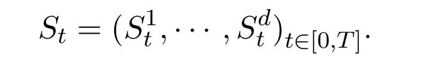
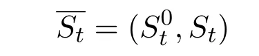
Throughout the paper,we fix arbitrarily anyT>0.Assume thatis a complete filtered probability space,and build a market model,which containsd+1 assets and the assets are priced at timet∈[0,T]withd∈N.At the same time,the terminal time isT.Here we divide thesed+1 assets into two categories:risky stocks and riskless bonds.Considerdrisky stocks and denote their price dynamics by the followingd-dimensional stochastic process,

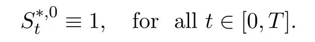
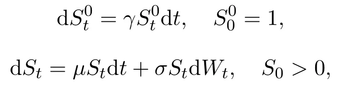
For the simplicity,about the riskless bonds,we only think one bond as the riskless bond.Here,it is denoted bywith a fixed interest rateγ>0.That is to say,,t≥0 and the initial capital.

Assume that the following formula

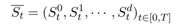
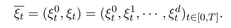
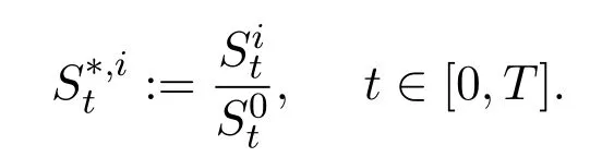
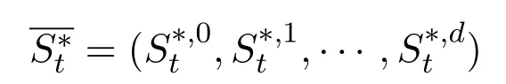
represents the corresponding price processes for this multi asset,which can be viewed as a vector-valued stochastic process.Generally speaking,we consideras a semi-martingale on the given filtered probability space.The non-negative randomrepresents the price of theithasset at timet.We also let

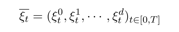
Recall a trading strategy which is an-predictableRd+1-valued process

Then,

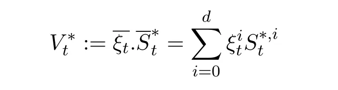
represents the value of the vector of the discounted assets prices at timet.

Note that,

Definition 2.1[10](Lemma 4.2.1)A trade strategy

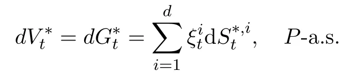
is called self-financing if the discounted value process

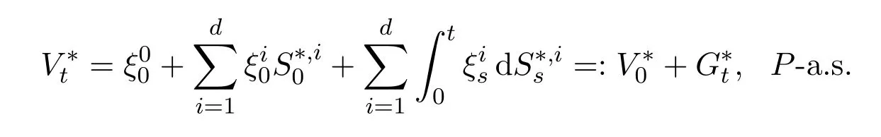
or equivalently in stochastic differential formulation

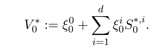
with initial data

Here,

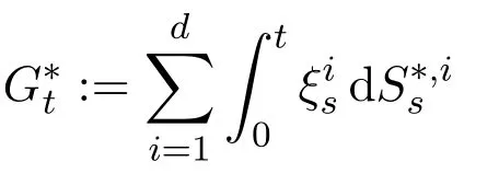
is the corresponding discounted gain process.

Definition 2.2A self-financing trading strategyis called an arbitrage opportunity ifsatisfies the following conditions:

(ii)?a constanta0so that;

Obviously,if such a strategy does not exist,then a model satisfies the no-arbitrage condition.

There are many examples,which show that the no-arbitrage condition cannot ensure the existence of an equivalent local martingale measure in the continuous-time setting.Such as the example in the reference[1](Example 7.7).Since that,we need a much stronger condition.Let us see the following no-arbitrage condition,which was introduced by Delbaen,Schachermayer and Shiryaer,and further considered by Shiryaev and Cherny[11].

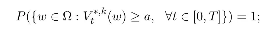
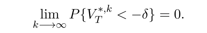
Definition 2.3[11](Definition1.6)We say that a sequence of self-financing trading strategiesrealises free lunch with vanishing risk condition,if the corresponding sequence of value processessatisfies that for eachk∈N:

(ii)there exists constantaksuch that

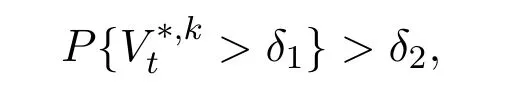
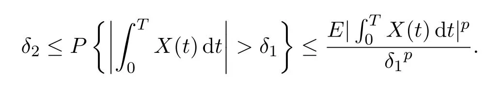
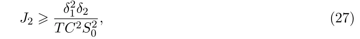
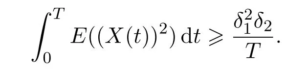
(iv)?constantsδ1,δ2>0(independent ofk)such that,.

Furthermore,if such a sequence of self-financing trading strategies does not exist,then the model statisfies the no free lunch with vanishing risk condition.

Definition 2.4We say that a sequence of self-financing trading strategies

satisfies the free lunch with bounded risk if it satisfies condition(i)and(ii)of Definition 2.3 as well as the following two conditions:

(i)there exists a constantasuch that,for eachk∈N,

(ii)there exists constantsδ1,δ2>0 such that,for eachk,

and for anyδ>0,

Obviously,if such a sequence strategies could not be found,then the model satisfies the no free lunch with bounded risk condition.

Theorem 2.1[1](Theorem1.1)(Fundamental Theorem of Asset Pricing)Assume that the asset price processis a locally bounded,(d+1)-dimensional vector-valued semi-martingale.Then there exists an equivalent local martingale measure forif and only if the no free lunch with vanishing risk condition holds.

2.2 The no good deal condition

Now we consider the no good deal condition.With the same preamble as before,we work on the same probability set-up.Following Biog-Nasal and Di Nunno[9],we assume that the givensatisfies that.We work in anL∞-framework and consider claims as elements of the spaceof random variables with finite norm.

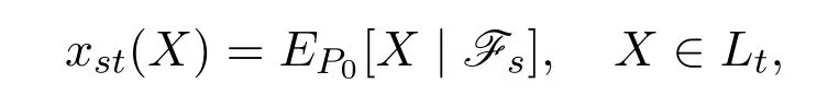
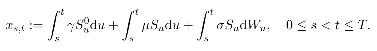
For any timet∈[0,T],letdenote the linear subspace representing all market claims that are payable at timet.At the same time,we work on a complete market,so that.For a given assetX∈Lt,we denote the systems of prices byxst,0≤s≤t≤T.We assume that pricexst(X),0≤s≤t≤T,for marked assetsX∈Ltare given and we describe them in axiomatic form,wherexst(X)denotes the price of assetXfromstot.Here,we set the bounds on prices:mst(X)≤xst(X)≤Mst(X)and we study the existence of a pricing measuresP0that allows a linear representation

fulfilling the given bounds.The pricing measureP0will reflect the choices of bounds.

Then let us focus on no good deal pricing measures.The good deal bound is a way to restrict the choice of equivalent martingale measures.And in incomplete markets,it often useQto denote.The idea is to consider martingale measures that not only rule out arbitrage possibilities,but also deals with “too good to be true”.As usual,we work with general price systems and not with specific price dynamics.Next let us introduce Definition 2.5.

Definition 2.5[9](Definition 6.1)A probability measureQ(equivalent toP)is called a no good deal pricing measure if there exists aδ>0 such that there are no good deals of levelδ>0 under Q(equivalent,for anyδ>0 there is no good deal of levelδ),i.e.

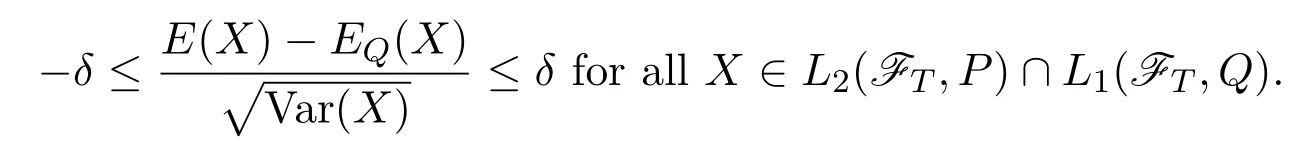
Justification of Definition 2.5According to Chicharee and Sa Requejo[15],a good deal of levelδ>0 is a non-negative-measurable payo ffX such that

Accordingly,a probability measureQequivalent to P is a no good deal pricing measure,if there are no good deals of levelδunderQ,i.e.

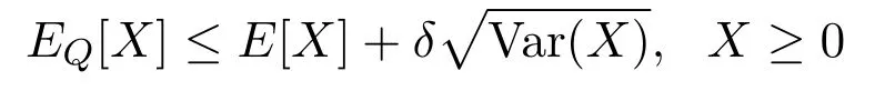
On the other hand,note that(1)holds for allX∈L∞(FT)as we haveX+∥X∥∞≥0.Hence,also the relation

3 Comparing two no-arbitrage conditions in index models

In this final section,we will focus on deriving the relationship between the two no-arbitrage conditions.Assumed,m∈Nbe fixed.We consider the following stochastic differential equation on[0,T]×Rd:

Where

andWtis an m-dimensional Brownian motion.Under the usual linear growth condition and the following Lipschitz condition:

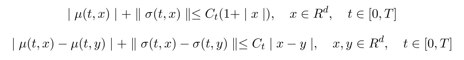
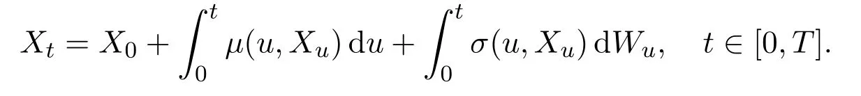
for some functionCt>0 ont∈[0,T],(2)has a unique strong solution(Xt)t≥0for a fixed original dataX0∈Rd,see,e.g.reference[12].

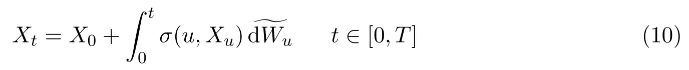
In the sequel,for the processXt,we use the following(equivalent)integral formulation,

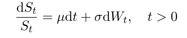
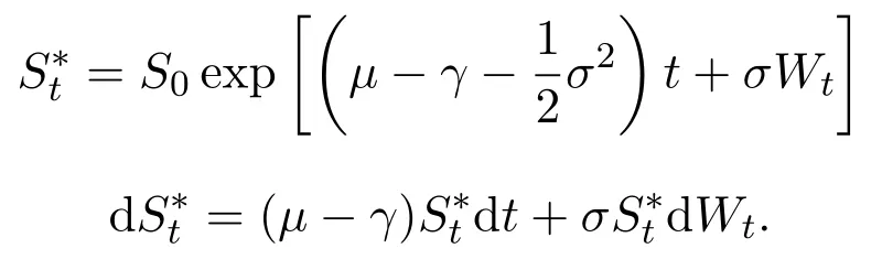
Now,let us think that the risk price process(St)t∈[0,T]is the one-dimensional special case,and it satisfies the following Black-Scholes pricing dynamics for a given initial priceS0>0,

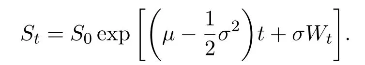
For given initial dataS0>0,using the Itformula(see,e.g.[12](Theorem 4.2.1)),one can derive that the risky assetStis determined uniquely by the above equation,andStis given explicitly by

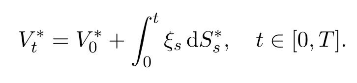
Let us clarify that the asset price process here isand according to Definition 2.1(with d=1),the discounted value process for a self-financing trading strategyis

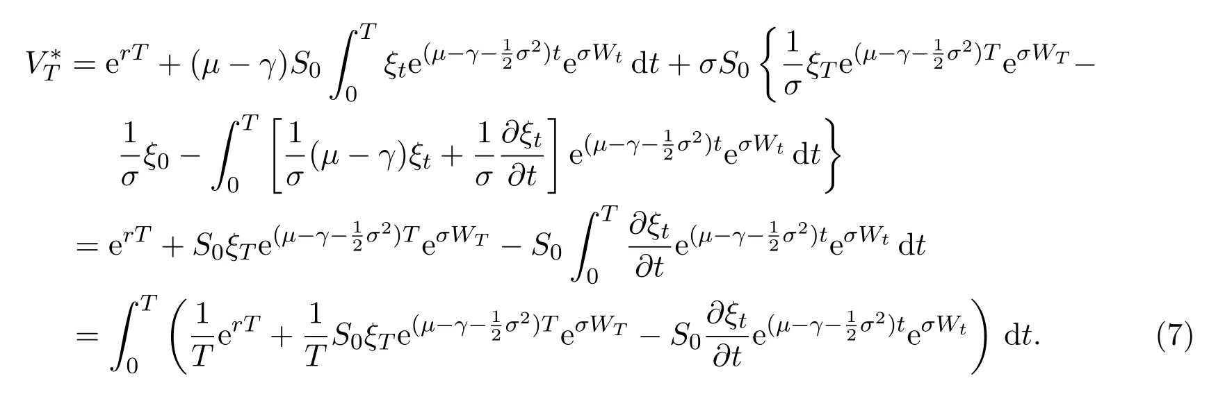
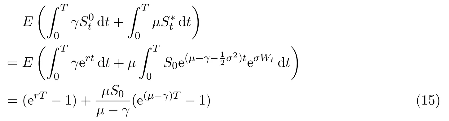
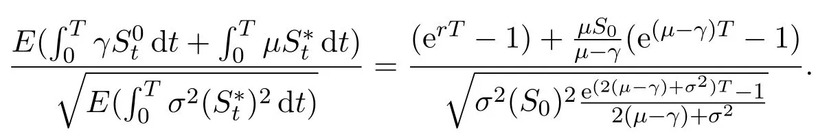
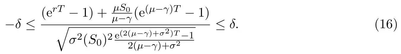
In this paper,we assume that the trading strategyis differentiable with respect tot.For making the comparison conditions neat,we letin our later discussion.In fact,V0?can be taken any non-negative constant and then use a constant to replace erT.

According to(4),the terminal discounted value for self-financing trading strategyis

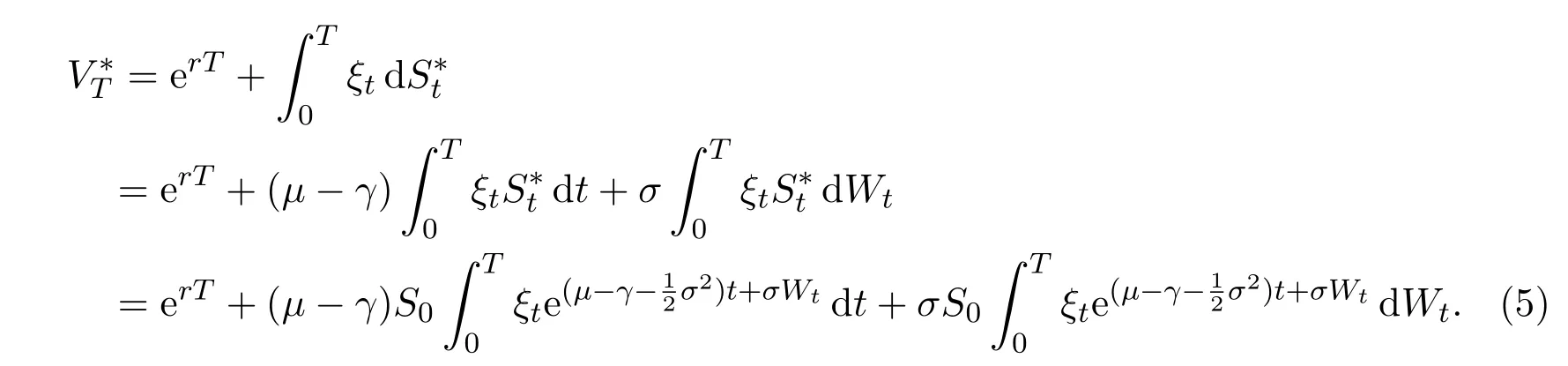
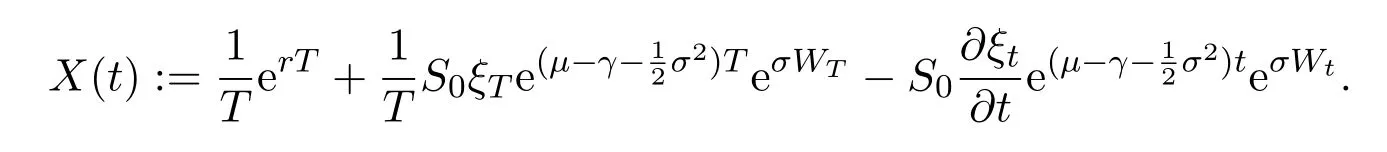
Let

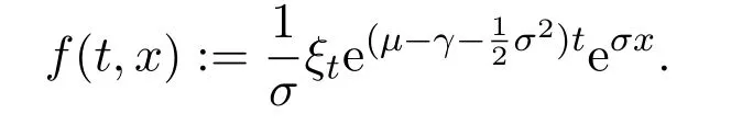
Then we get

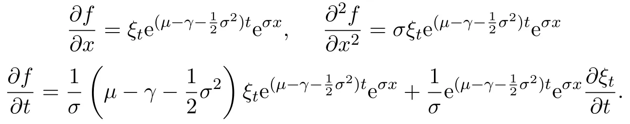
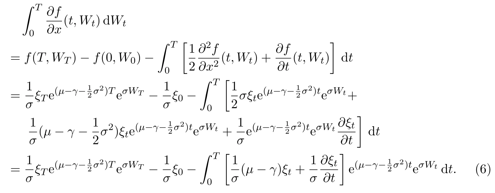
Taking formula(6)into equation(5),we get

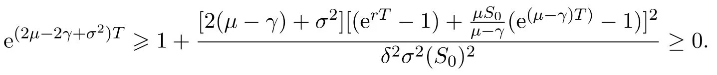
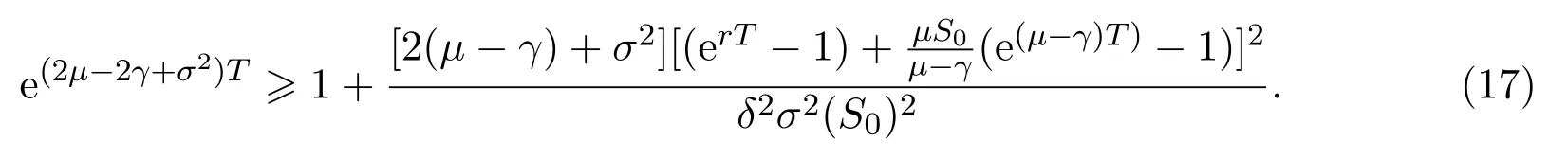
Assume that

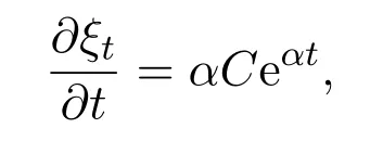
In this paper,we letξt=Ceαtsimulate the real market.In fact,real markets are complex and the assets cannot change linearly.So we fit that the asset are changing exponentially.At the same time,ifα≥0,we can say that the assets grow exponentially.On the contrary,ifα<0,we say that the assets are falling exponentially.Now letξt=Ceαt,then

so we get that:

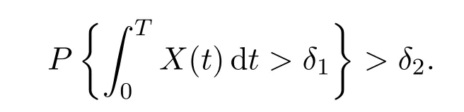
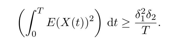
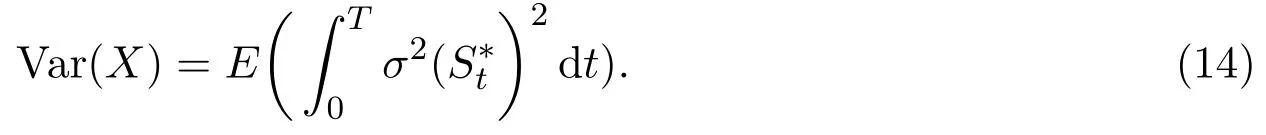
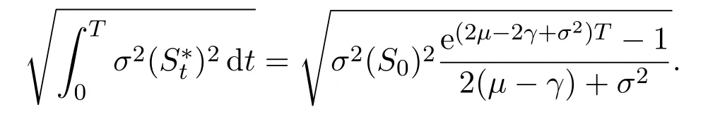
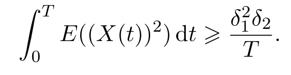
Recall Definition 2.3(iv),there exist constantsδ1,δ2>0 such that

For anyp>0,by Chebyshev′s inequality,

For anyp,q>1 and,

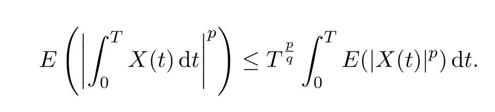
More generally,whenp=q=2,we get

Then,evaluate each of these in terms ofdt.(By the identity

We first have the following:

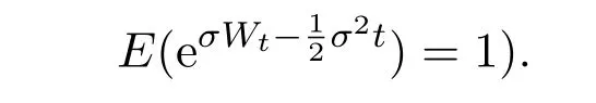
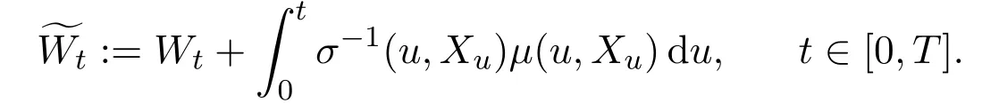
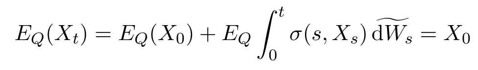
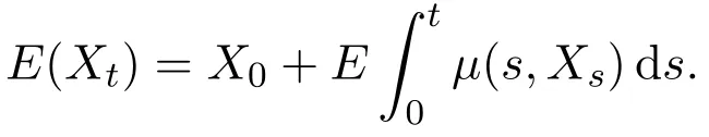
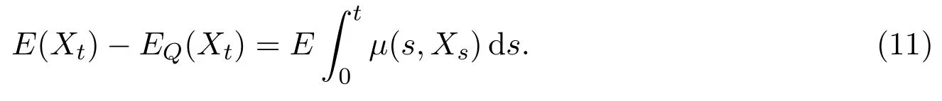
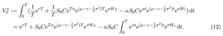
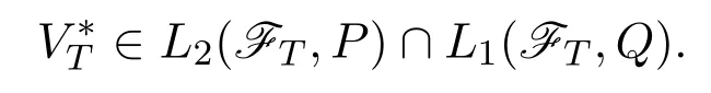
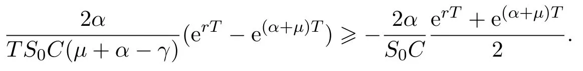
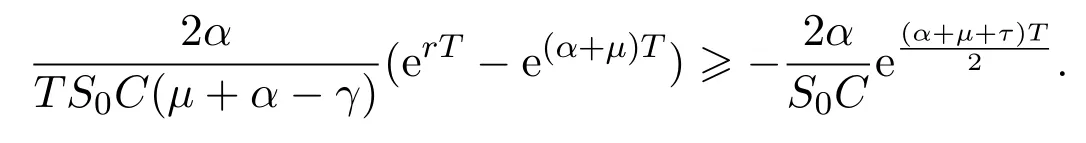
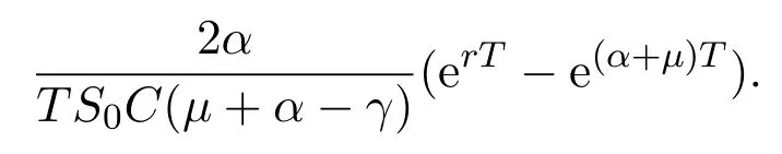
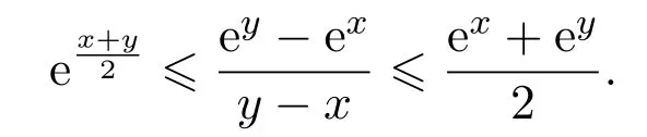
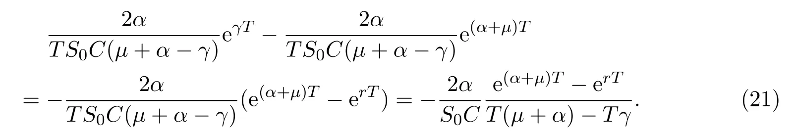
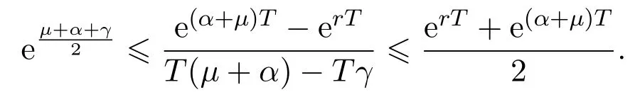
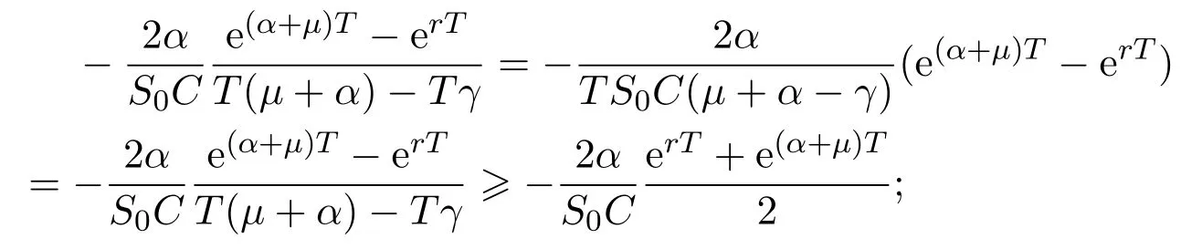
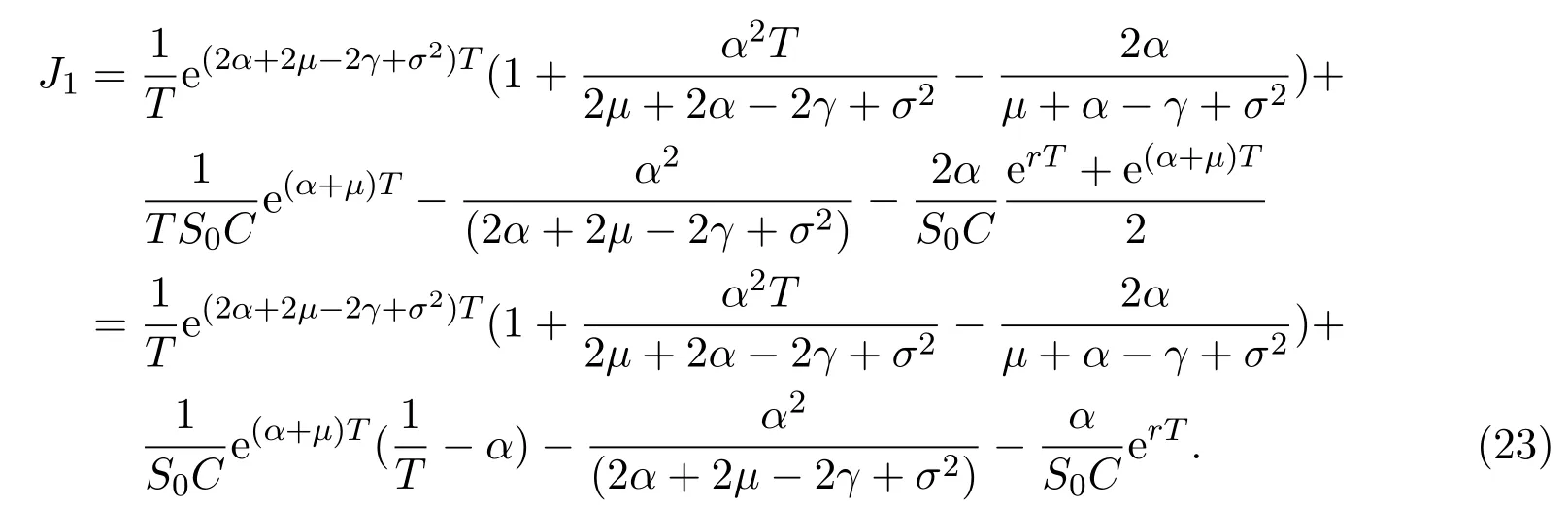
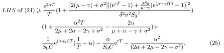
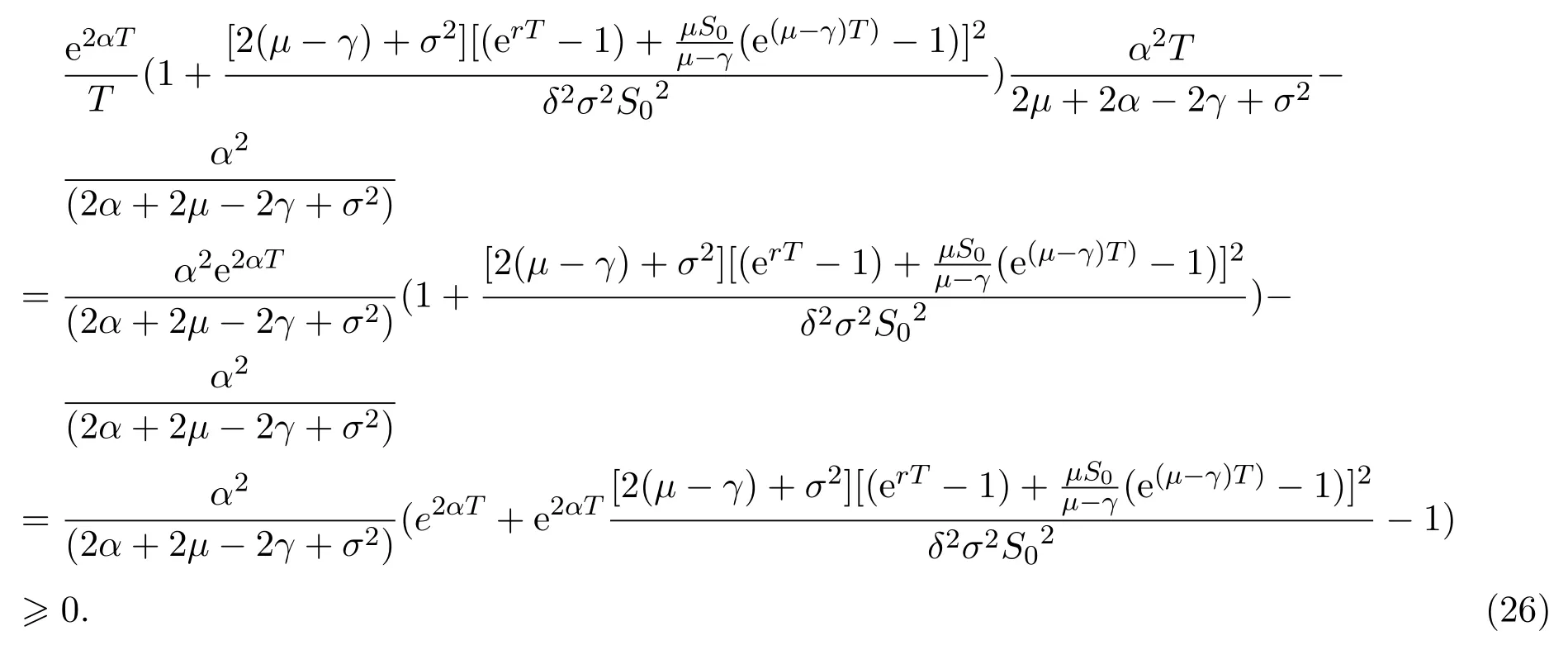
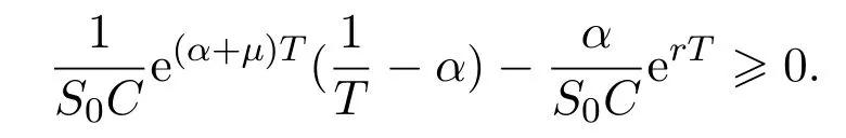
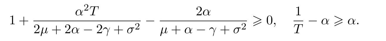
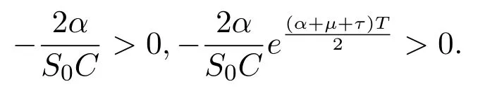
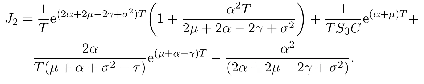
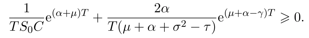
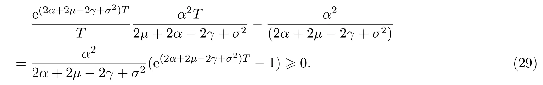
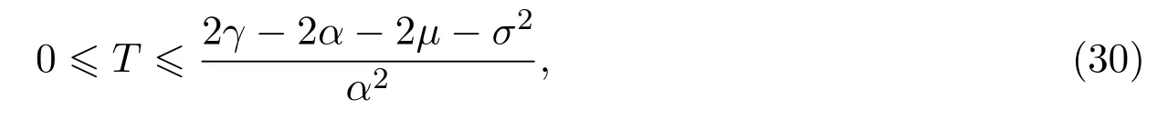
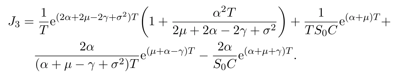
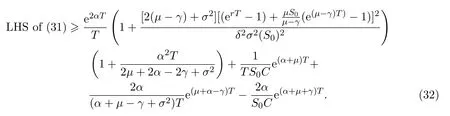
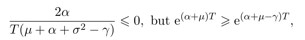
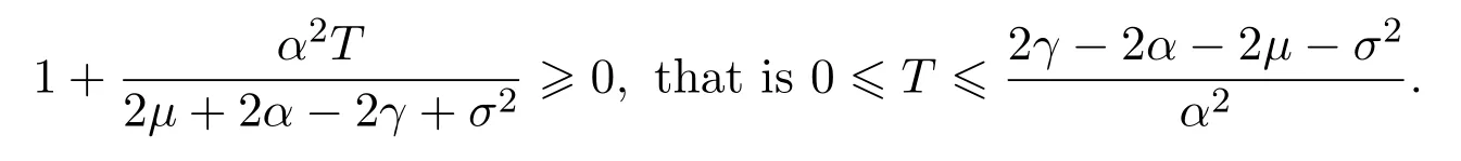
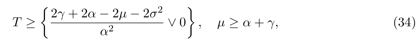
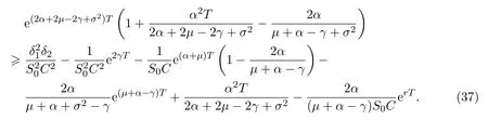
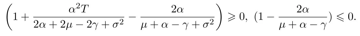
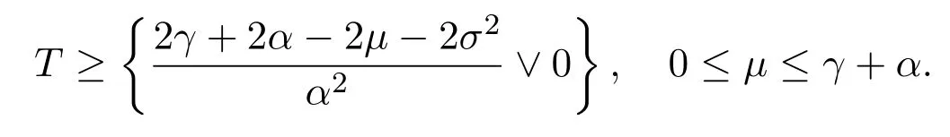
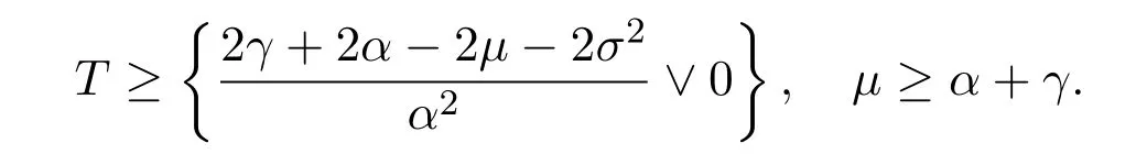
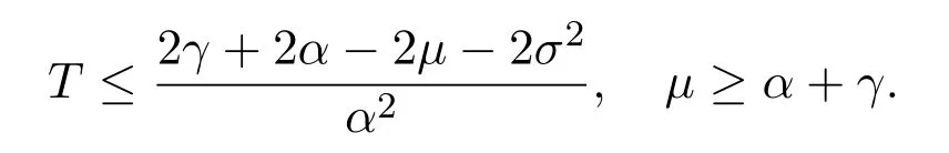
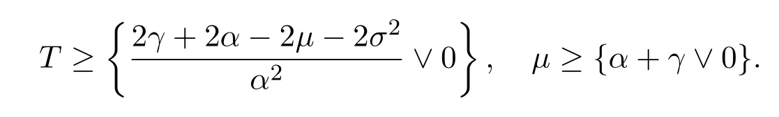
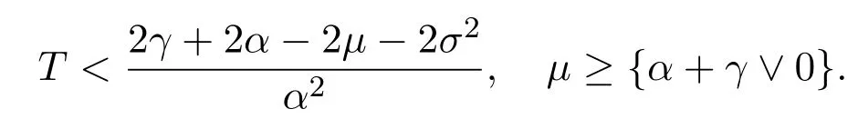
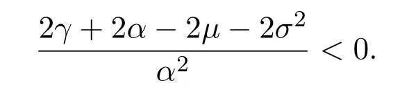
In addition,let′s consider the no good deal condition.According to the previous definition,we know that the price is given by the system{xs,t}0≤s

Define that

According to reference[13],we get

with

Next,defineQvia

Then by the Girsanov theorem,we know thatis aQ-Brownian motion.

Let us take the expectation of both sides of(10)

and

Thus

Next,we turn to the special case of the(previously introduced)asset price process

for

We have the associatedxs,tdefined as follows:

Recall(3)and(4),namely,

Recall(7),forξt=Ceαt,the discounted terminal value

Obviously,

Using the identity

let the payo ff

Then,we get

and

Calculate(13)and(14):

and

Recall the Definition 2.5 and by(13)-(14),we get the following equation:

Finally,we obtain the no good deal condition as follows:

Proposition 3.1When the condition 2μ?2γ+σ2>0 holds,then

Moreover,we get that:

1)Ifα≥0,then

2)Ifα<0,then

ProofWe first note that(16)can be reduced to

Whetherα≥0 orα<0,e2αT>0.So,we have

Let us assume that the right-hand side(RHS)of(18)>0.Then it is easy to find

Next we scale down the following expression(Notice that it is the part of the transformation from the(8))

We consider

It is well known that the logarithmic mean lies between the geometric mean and the arithmetic mean[14].

Thus,fors,t>0,with.Thus,if we lets=ex,t=eyforx,y∈?with,we get

With this in hand,we continue to calculate the following formula

So,we have

Furthermore,we have

Theorem 3.1Letα>0 and 2μ?2γ+σ2≥0.Assume that

then condition(16)can imply condition(8),which indicates that the no good deal condition for fundamental theorem is stronger than the no free lunch with vanishing risk condition.

ProofWe have known that 2μ?2γ+σ2≥0.Ifα>0,it is easy to know that 2α+2μ?2γ+σ2>0,μ+α?γ+σ2>0.Recall(20),and we apply proposition 3.1 to(20).At the same time,we need to get rid of some positive terms to shrink(20),so we delete the.Thus we let

Let us assume that the right-hand side(RHS)of(25)>0.In fact,α,μ,γ>0,and e2αT>1.

And we get that

Then we can get

Therefore,we know that ifα≥0,2μ?2γ+σ2≥0,under condition(22),condition(16)can imply condition(24).As condition(24)is stronger than condition(8),we then verify that condition(16)implies condition(8).

Theorem 3.2Whenα<0,2μ?2γ+σ2≥0,2μ+2α?2γ+σ2>0,then we know that condition(16)can implies condition(8),which indicates that the no good deal condition for fundamental theorem is stronger than the no free lunch with vanishing risk condition.

ProofForα<0,2μ?2γ+σ2≥0,then

If 2μ+2α?2γ+σ2>0,then we can know that.We apply proposition 3.1 to(20).At the same time,we need to get rid of some positive terms to shrink(20),so we delete the

Let

then

Obviously,(27)is stronger than(8).If(16)is true,then by putting(18)into the left-hand side(LHS)of(27),it yields that

Let us assume that the right-hand side(RHS)of(28)>0.In fact,forμ,γ>0,we then have

So,we get

At the same time,2μ+2α?2γ+σ2>0,so that e(2μ+2α?2γ+σ2)T>1.

Moreover,

So,underα<0,2μ?2γ+σ2≥0,2μ+2α?2γ+σ2>0,condition(16)can imply condition(27).As condition(27)is stronger than condition(8),we know that condition(16)implies condition(8).

Theorem 3.3Letα<0,2μ?2γ+σ2≥0,and 2μ+2α?2γ+σ2<0.If

then condition(16)implies condition(8),which indicates that the no good deal condition for fundamental theorem is stronger than the no free lunch with vanishing risk condition.

ProofIf 2μ+2α?2γ+σ2<0,μ+α?γ+σ2>0,we apply proposition 3.1 to(20).At the same time,we need to get rid of some positive terms to shrink(20),so we delete the

Let

then

Clearly,(31)is stronger than(8).If(16)is true,then by taking(18)into the left-hand side(LHS)of(31),it yields that

Let us assume that the right-hand side(RHS)of(32)>0.Then,forμ,γ>0,we have

it is exponential growth.So,we need,then we can get

Thus,we get that ifα<0,2μ?2γ+σ2≥0,2μ+2α?2γ+σ2<0,μ+α?γ+σ2>0,under condition(30),condition(16)can imply condition(31).Because condition(8)is weaker than condition(31),we then verify that condition(16)implies condition(8).

When the caseα<0,2μ+2α?2γ+σ26 0,μ+α?γ+σ2<0,no condition that satisfy this situation can be found,thus we just leave it out here.

Becauseξt=Ceαt,we should useα≥0 orα<0 to match the rise and fall of the market.Thus we shrink(20)intoJ1,J2andJ3.At the same time,this is the point of innovation in this paper and the difference from the linear models.

From the discussion above,we know that if Theorem 8,Theorem 9 or Theorem 10 holds,then the no good deal condition can implies the no free lunch with vanishing risk condition.

On the other hand,let′s consider whether condition(8)implies condition(16).That is to say,under what conditions the no free lunch with vanishing risk condition can imply the no good deal condition.

Becauseμ>0,γ>0,andα∈R,we classifyα∈Rinto two cases:α≥?μandα

Theorem 3.4We get that:

1.The case thatα+μ≥0,

(a)Ifα+μ?γ≥0,under the condition

then(8)can imply(16).

(b)Ifα+μ?γ<0,α+μ?γ+σ2≥0,under the condition

then(8)can imply(16).

(c)Ifα+μ?γ<0,α+μ?γ+σ2<0,under the condition

then(8)can imply(16).

2.The case thatα+μ<0,α+μ?γ+σ2>0,under the condition

then(8)can imply(16).

That means under the conditions(33)-(36)the no good deal condition for fundamental theorem is weaker than the no free lunch with vanishing risk condition.

ProofAssume that(8)is true.Then we have

Let RHS of(37)>0,we need

1.Letα≥?μ,that is to sayα+μ≥0.

(a)Ifα+μ?γ≥0,then it is easy to see thatα+μ?γ+σ2≥0.

Then,the solution to(37)is

(b)Ifα+μ?γ<0,α+μ?γ+σ2≥0,then the solution to(37)is

(c)Ifα+μ?γ<0,α+μ?γ+σ2<0,then the solution to(37)is

2.Letα

(a)Ifα+μ?γ+σ2≥0,then the solution to(37)is

(b)Ifα+μ?γ+σ2<0,then the solution to(37)is

But

In fact,T>0,so we clearly know that it can not happen.