Parameter estimation for dynamical systems based on improved differential evolution algorithm
2019-01-12 05:41:08MinTaoHuChaolong
純粹數學與應用數學 2018年4期
Min Tao,Hu Chaolong
(School of Science,Xi′an University of Technology,Xi′an 710048,China)
Abstract:In computational science it is common to describe dynamic systems by mathematical models in forms of differential.These models may contain parameters that have to be computed for the model to be complete.In the present study,we have developed a improved differential evolution for parameter estimation for time varying dynamical systems.Numerical experiments are presented to show the efficiency of the proposed method.
Keywords:differential evolution,parameter estimation,dynamical systems,ordinary differential equations
1 Introduction
Parameter estimation is widely used in modeling of dynamic processes in physics,engineering and biology etc[1-3].Various methods have been previously investigated in the literature for handing this problem.The classical methods for dealing with parameter identification problem such as Nelder-Mead[4],Gauss-Newton[5]and smoothing the data method[6-8]can achieve reasonably good solutions for parameter identification of smaller sizes.But they are insufficiently robust for complex problems involving huge search space and they are lack of ability to overcome the local optimum points and reach the global optimum.In the recent years,evolutionary algorithms like genetic algorithms(GA)[9-11],particle swarm optimization(GA)[12]and differential evolution algorithms(DE)[13-15]have also been used for solving such problems.One of the main advantages to using these techniques is that they require no knowledge or gradient information about the response surface.In the present study,we propose a improved differential evolution algorithm to solve parameter estimation problems.Our approach uses a penalty function and a logic function based on feasibility to guide the search to the feasible region.The proposed approach does not require any extra parameters other than those normally adopted by the differential evolution algorithms.From the illustrated example it can be seen that this method is effective and result is satisfactory.
The paper is organized as follows:introduction of parameter identification problem is given brie fly in section 2.Section 3 describes the improved differential evolution algorithms used in this study.Examples are given in order to illustrate the effectiveness of the proposed method is given in Section 4.Finally the conclusions based on the present study are drawn in section 5.
2 Parameter identification problem
Let us assume the mathematical model of dynamical systems is described by the ordinary differential equations of the form
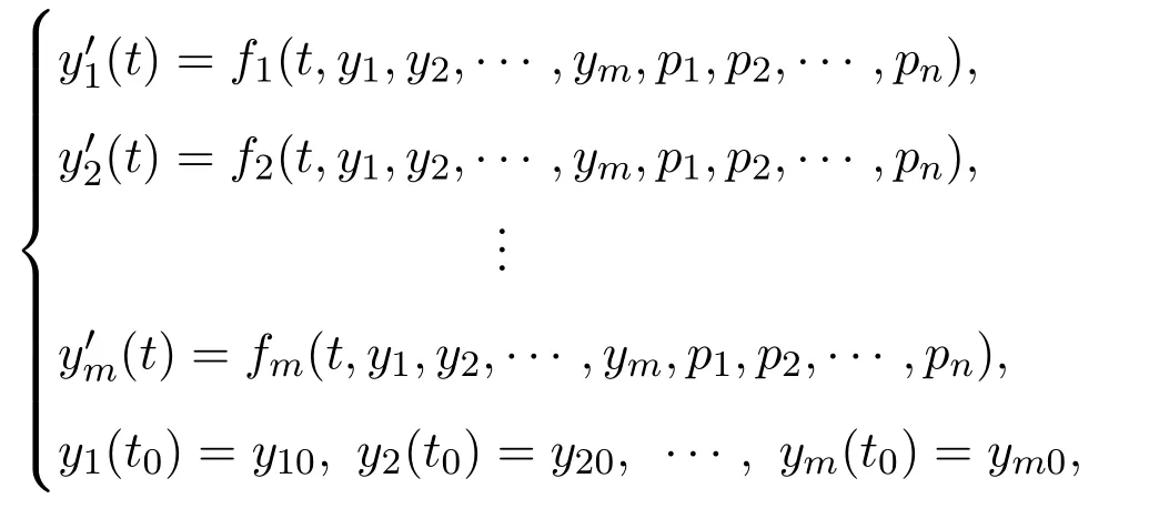
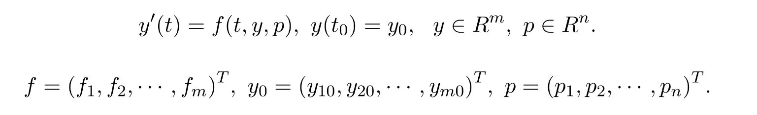
wherep1,p2,···,pnis the vector ofnunknown real parameters,y10,y20,···,ym0are the initial values of the system,the functionsfi(i=1,2,···,m)are known,y=(y1(t),y2(t),···,ym(t))is the state vector of the system.Written in vector form as
In addition,experimental data set are given from(ti,y(i)),i=1,2,···,k,wheretirepresents the independent variable andy(i)is the measured value of the corresponding dependent variable.Usuallyn?k,the problem we consider here is to estimate the optimum parameter vectorp?as accurate as possible using the given experimental data,and this is a minimization problem which can be defined by
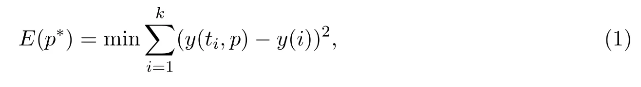
wherey(ti,p)andy(i)are the numeric solution of the mathematical model and experimental data point for thei-th data point,respectively.
3 Improved differential evolution algorithm
In this section we will describe brie fly the working of basic differential evolution and improved differential evolution algorithms.
Generally,a multi-constrained nonlinear optimization problem can be expressed as follows:

whereLi≤xi≤Ui,i=1,2,···,n.
Here,nis the number of the decision or parameter variables,thei-th variable variesxiin the range[Li,Ui].The functionis the objective function.The decision or search spaceSis written as
3.1 The basic DE algorithm
Let′s suppose that
are solutions at generation
is the population,whereDis the population size.In DE,the child populationPl+1is generated through the following operators.
1)Mutation operator For eachin parent population,the mutant vectoris generated according to the following equation:
wherer1,r2,r3∈{1,2,···,D}iare randomly chosen and mutually different,the scaling factorxfcontrols amplification of the differential variation.
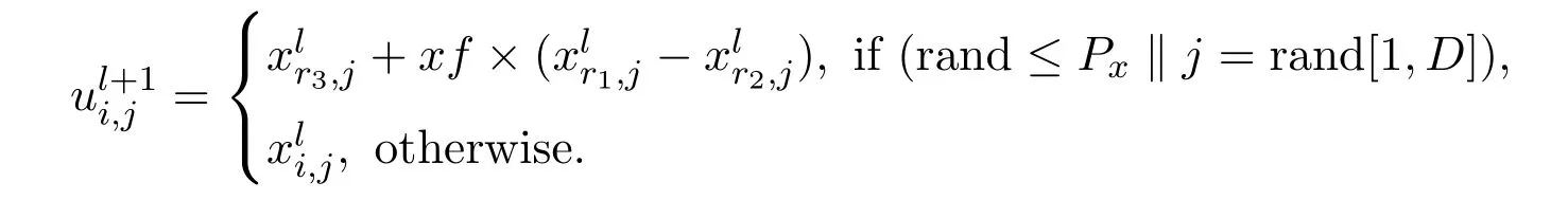
2)Crossover operator For each individual,a trial vectoris generated by the following equation:
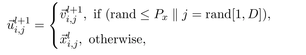
where rand is a uniform random number distributed between 0 and 1,rand[1,D]is a randomly selected index from the set{1,2,···,N},Px∈[0,1]controls the diversity of the population.
3)Selection Operator The child individualis selected from each pair ofandby using greedy selection criterion:
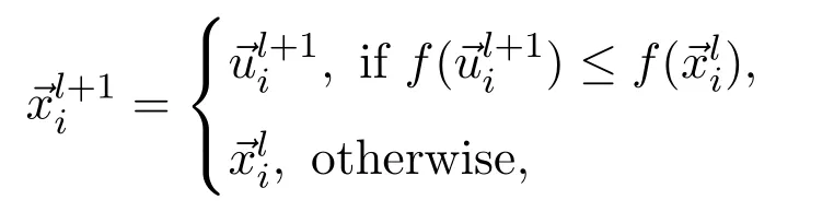
where the functionfis the objective function and the conditionmeans the individualis better than.The above-mentioned three steps are repeated generation by generation until the specific termination criteria are satisfied.
3.2 Improved differential evolution algorithm
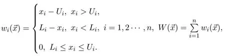
It is important to notice that the reproduction operation of DE is able to extend the search outside of the initialized range of the search space.It is also worthwhile to notice that sometimes this is beneficial property in problems with no boundary constraints because it is possible to find the optimum that is located outside of the initialized range.However,in boundary constrained problems,it is essential to ensure that parameter values lie inside their allowed ranges after reproduction.A simple way to guarantee this is to define a penalty function as follows:
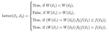
Defining logic function as follows:
The improved differential evolution algorithm procedure is described as follows:
Step1Randomly generate initial groups in searching space,whereDis the population size,Pxis Crossover probability,xfis Cross factor.
Step2Setl=0.

Step3Iflis bigger than maxGen then break,else.
Step4Arrange the groupsPlfrom better to worse according to logic function better,it is still remarked asis the best individual andis the worst individual.
Step5If betteris real(the best individual and the worst individual are the same),go to Step8.
Step6For each individualin the populationPl,generate three random integersr1,r2andr3∈{1,2,···,D}i,with,generate a random integerjrand∈{1,2,···,D}for each parameterjdo
Step7Replacewith the childin the populationifis better,otherwise,go to Step3.
Step8Output the best solutions including all the solutions which cause the function′s value to be the minimum value.
4 Numerical results
In the parameter identification problem the parameters which are to be determined and optimized are randomly generated within the given range,for example,,where,Dis the population size.After each iteration,the new valuesfor each possible solution ofare determined using the Runge-Kutta method and fitness of each individual is determined using equation(1).In the follow example,3 independent runs are made which involves 3 different initial trial solutions with randomly generated a population is set to 10×n,wherenis dimension of the problem,a crossover probabilityPxequal to 0.2,the scaling factorxfof 0.8.The termination criterion has been set limited to a maximum number of generations.
Example 1Irreversible liquid-phase reaction of the first order.
The first example is a parameter estimation problem with two parameters and two differential equations.It was published in Esposito and Floudas[1].
It involves a first-order irreversible isothermal liquid-phase chain reaction.
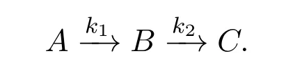
The problem can be formulated as follows:
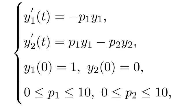
wherey1andy2are the mole fractions of components A and B,respectively.p1andp2are the rate constants of the first and second reaction,respectively.yi(tj)is the experimental point for the state variableiat timetj.The experimental data are used taken from Esposito and Floudas[1],and given in Table 1.
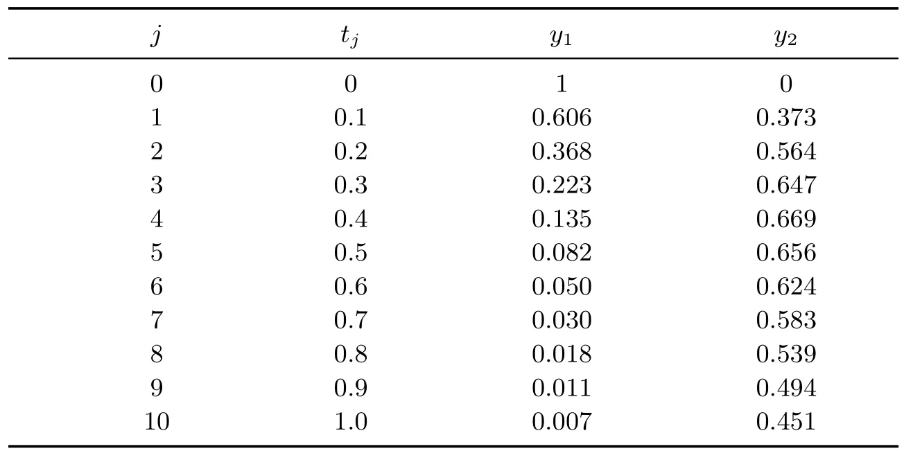
Table 1 Data for irreversible liquid-phase reaction problem
In this experimental study,the improved differential evolution algorithm are set as follows:the population size 10×2,a crossover probabilityPxequal to 0.2,the scaling factorxfof 0.8.Table 2 gives the results for problem 1 taken by fixing the maximum number of generation 100,200,the last column of the table which give the sum of square error(SSE).Plot of experimental data and data obtained by improved differential evolution after 200 generation is given in Figure 1.
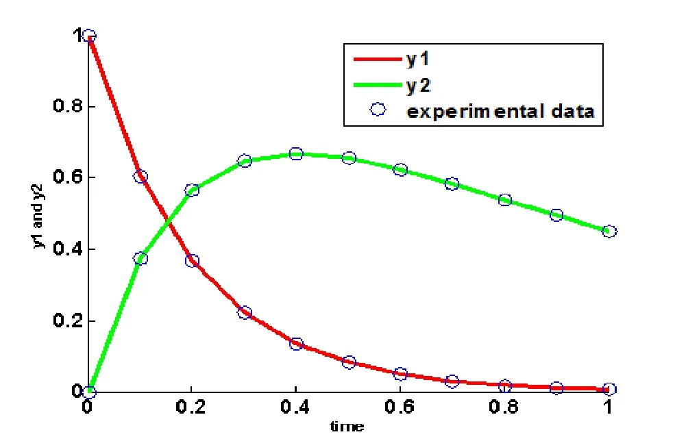
Figure 1 Irreversible Liquid-phase Reaction model at 200 generation

Table 2 Results obtained using improved differential evolution algorithm
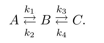
Example 2Reversible liquid-phase reaction of the first order.
The second example is a parameter estimation problem with four parameters and three differential equations.It appears in Esposito and Floudas[1].
It involves a first-order reversible isothermal liquid-phase chain reaction.
The problem can be formulated as follows:
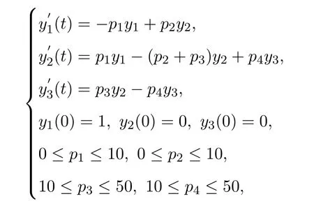
wherey1,y2andy3are the mole fractions of components A,B and C,respectively.p1,p2andp3are the rate constants of the first and second reaction,respectively.yi(tj)is the experimental point for the state variableiat timetj.The experimental data are used taken from Esposito and Floudas[1]and given in Table 3.
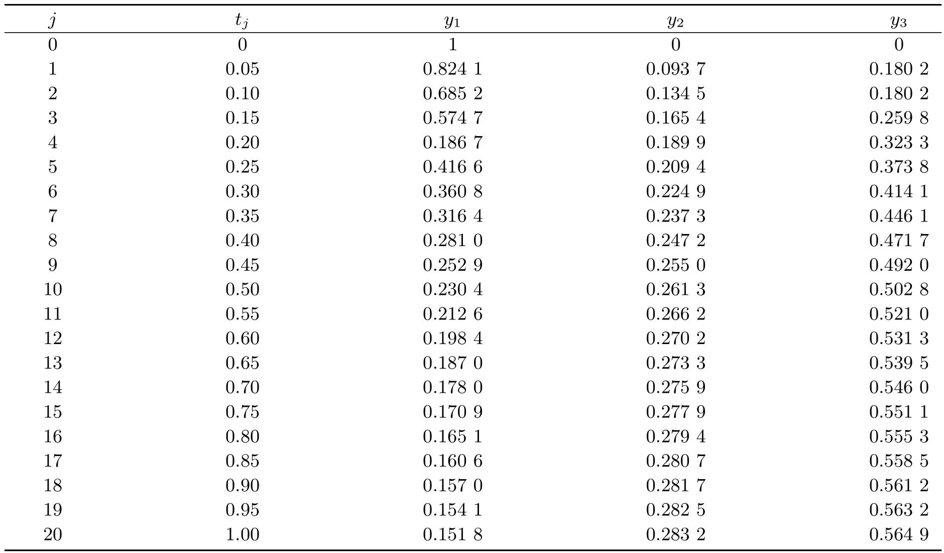
Table 3 Data for reversible liquid-phase reaction problem
In this experimental study,the improved differential evolution algorithm are set as follows:the population size 10×4,a crossover probabilityPxequal to 0.2,the scaling factorxfof 0.8.Table 4 gives the results for problem 2 taken by fixing the maximum number of generation 100,200,the last column of the table which gives the sum of square error(SSE).Plot of experimental data and data obtained by improved differential evolution after 200 generation is given in Figure 2.
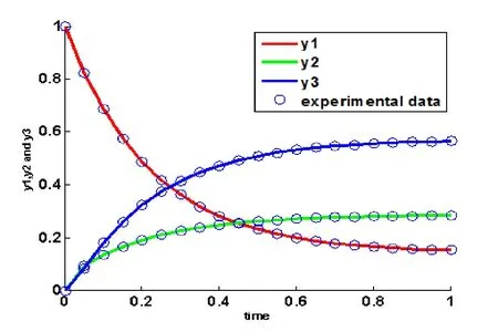
Figure 2 Reversible Liquid-phase Reaction model at 200 generation
From Table 2,Table 4 and Figure 1-Figure 2,it can be concluded that the proposed improved differential evolution algorithm can give a more effective and robust way for finding the actual parameters in the given range.
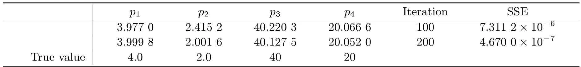
Table 4 Results obtained using improved differential evolution algorithm
5 Conclusions
In this paper,a improved differential evolution algorithm is proposed for solving parameter identification problems.From the illustrated example,it can be seen that the proposed numerical method is efficient and accurate to estimate the parameter of mathematical model.
Generally speaking,the population size,the crossover probabilityPx,the scaling factorxfand the maximum number of generation are primary factors influencing the implementation of the algorithm.However,by computations for the simultaneous inversion problem,we find that the population size is set 10×n,wherenis dimension of the problem,a crossover probabilityPxequal to 0.2,the scaling factorxfof 0.8,the termination criterion has been set limited to a maximum number of 200 generations,the parameter estimation effect is best.