SLOW MANIFOLD AND PARAMETER ESTIMATION FOR A NONLOCAL FAST-SLOW DYNAMICAL SYSTEM WITH BROWNIAN MOTION?

School of Mathematics and Statistics,Huazhong University of Science and Technology,Wuhan 430074,China

Center for Mathematical Sciences,Huazhong University of Science and Technology,Wuhan 430074,China E-mail:hinazul fiqar@hust.edu.cn

Ziying HE (賀紫盈)

School of Science,Wuhan University of Technology,Wuhan 430074,China Center for Mathematical Sciences,Huazhong University of Science and Technology,Wuhan 430074,China E-mail:ziyinghe@whut.edu.cn

Meihua YANG (楊美化)

School of Mathematics and Statistics,Huazhong University of Science and Technology,Wuhan 430074,China E-mail:yangmeih@hust.edu.cn

Jinqiao DUAN (段金橋)

Department of Applied Mathematics,Illinois Institute of Technology,Chicago,IL 60616,USA Center for Mathematical Sciences,Huazhong University of Science and Technology,Wuhan 430074,China E-mail:duan@iit.edu

Abstract We establish a slow manifold for a fast-slow dynamical system with anomalous diffusion,where both fast and slow components are in fluenced by white noise.Furthermore,we verify the exponential tracking property for the established random slow manifold,which leads to a lower dimensional reduced system.Alongside this we consider a parameter estimation method for a nonlocal fast-slow stochastic dynamical system,where only the slow component is observable.In terms of quantifying parameters in stochastic evolutionary systems,the provided method offers the advantage of dimension reduction.

Key words Nonlocal Laplacian;fast-slow system;stochastic system;random slow manifold;exponential tracking property;parameter estimation

1 Introduction

For investigating dynamical behaviours of deterministic systems,the theory of invariant manifolds has a popular history.Hadamard[23]introduced it for the first time;it was then addressed by Lyapunov and Perron[8,12,17].For a deterministic system it has been modi fied by numerous authors[5,11,13,18,24,34].Duan and Wang[19]explained effective dynamics for the stochastic partial differential equations.Schmalfu? and Schneider[36]recently explored random inertial manifolds for stochastic differential equations with two times scales by a fixed point technique,where they eliminate the fast variables via random graph transformation.They showed that as the scale parameter approaches zero,the inertial manifold approaches some other manifold,de fined in terms of a slow manifold.Wang and Roberts[37]explored the averaging of a slow manifold for fast-slow stochastic differential equation,in which only the fast mode is in fluenced by white noise.For multi-time-scale stochastic systems,the exploration of slow manifolds was conducted by Fu,Liu and Duan[22].Bai et al.[4]recently established the existence of a slow manifold for nonlocal fast-slow stochastic evolutionary equations in which only the fast mode is in fluenced by white noise.Ren et al.[33]devised a parameter estimation method based on a random slow manifold for a finite dimensional slow-fast stochastic system.

The fundamental objective of this paper is to establish the existence of random invariant manifold

M

,for small enough

?>

0,with an exponential tracking property(Section 4),and to conduct a parameter estimation by using observations only on the slow system for a nonlocal fast-slow stochastic evolutionary system(Section 5).Since the slow system is lower dimensional compared to the original stochastic system,in terms of computational cost this parameter estimator offers a bene fit.In addition,it provides the advantage of using the observations only on slow components.We verify the results regarding the slow manifold,exponential tracking property and parameter estimation in last section,via theoretical example and an example from numerical simulation.Before constructing the invariant manifold,we need to prove the existence and then the uniqueness of a solution for system(1.1)–(1.2).This is done in the next section.Many nonlocal problems explained in[6]are similar to our nonlocal system.There are usually two techniques for the establishment of invariant manifolds:the Hadamard graph transform method[18,35]and the Lyapunov-Perron method[8,12,17].For the achievement of our objective we used the Lyapunov method,which is different from the method of random graph transformation.More speci fically,it can be shown that the established manifold

M

can be asymptotically approximated to a slow manifold

M

for sufficiently small

?

,under suitable conditions.

In the present paper,we explore the following nonlocal fast-slow stochastic evolutionary system:

Here,

u

is in

H

,

v

is in

H

,

u

|(?1

,

1)=0,

v

|(?1

,

1)=0.We set

H

=

L

(?1

,

1),which denotes the space for fast variables,while

H

is some generic separable Hilbert space,which denotes the space for slow variables.Linear operator

J

,and nonlinear interaction functions

f

and

g

,will be speci fied in the next section.The constants

σ

and

σ

are white noise intensities.For

x

∈R,

α

∈(0

,

2)

,

is called a fractional Laplacian operator,which is a nonlocal operator with the Cauchy principle value(P.V.)considered to be the limit of the integral over R(

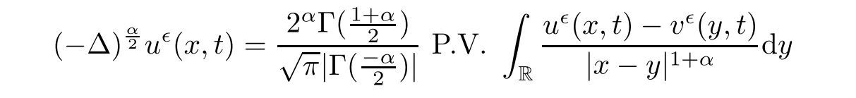
x

?

?,x

+

?

)for

?

tending to zero.The Gamma function is de fined as

The state space for system(1.1)–(1.2)is a separable Hilbert space H=

H

×

H

.

Here

H

is a space of square integrable functions on(?1

,

1);it follows that

H

=

L

(?1

,

1)and that

H

is some generic separable Hilbert space.Norms‖·‖and‖·‖are considered to be the norms of

H

and

H

,respectively.The norm of separable Hilbert space H is de fined as

In system(1.1)–(1.2),

?

is a small parameter with the bound 0

<?

?1,

u

is a fast component and

v

is a slow component.

We introduce a few fundamental concepts in random dynamical systems and nonlocal or fractional Laplacian operators in the next section.

2 Preliminaries

De finition 2.1

([16])A stochastic process{

W

(

ω

):

t

≥0}de fined on a probability space(?

,

F

,

P)taking values in a Hilbert space is called a one sided Wiener process if the following conditions hold:?

W

=0 a.s.;?the paths

t

→

W

(

ω

)are continuous,a.s.;?

W

has independent increments,that is,if 0≤

t

<t

<t

<

···

<t

,then the random variables

W

?

W

,

···

,W

?

W

are independent;?

W

has stationary increments that are Gaussian distributed.

In order to use random dynamical systems techniques,we should take

W

and

W

in equations(1.1)–(1.2)to be two-sided in time.This can be done as follows:

De finition 2.2

([3])Let(?

,

F

,

P)be a probability space and let

θ

={

θ

}be a flow on ?;that is,a mapping

which satis fies the following conditions:

?

θ

=

Id

;?

θ

θ

=

θ

,

where

r

,r

∈R;

To achieve our objective,we take a special but very important driving dynamical system in fluenced by the Wiener process.Let us consider

W

(

t

),taking values in state space(Hilbert space)H to be a two-sided Wiener process which depends upon time

t

and also varying with

t

.The de fined Wiener process has zero value at

t

=0.Its sample path is the space of real continuous functions on R,which is denoted by

C

(R

,

H).Here we take the flow,which is also measurable and de fined by

θ

={

θ

},as

On B(

C

(R

,

H)),the distribution of the above process induces a probability measure,which is known as the Wiener measure.Instead of the whole

C

(R

,

H),we consider an{

θ

}invariant subset ??

C

(R

,

H)whose probability-measure is one.With respect to ?,we also take the trace

σ

-algebra F of B(

C

(R

,

H)).Recalling the concept of{

θ

}-invariant,a set ?is said to be{

θ

}-invariant if

θ

?=?.Here we take the restriction of the Wiener measure and we still represent it by P

.

On the state space H(which is often taken as a Hilbert space),the dynamics of a stochastic system over a flow

θ

is depicted by a cocycle in general.

De finition 2.3

([3])A cocycle

φ

is de fined by the map

which is(B(R)?F?B(H)

,

F)-measurable and satis fies the conditions

for

y

∈H,

ω

∈? and

r

,r

∈R.Then

φ

,together with metric dynamical system(?

,

F

,

P

,θ

),constructs a random dynamical system.

is a random variable.This family is then said to be a random set.

De finition 2.4

([16])A random variable

y

(

ω

)

,

which takes values in H,is known as a stationary orbit(random fixed point)for a random system

φ

if

for all

r

.

Now the idea of the random invariant manifold is given.

De finition 2.5

([22])If a random set

M

={

M

(

ω

):

ω

∈?}satis fies the condition

for

ω

∈? and

r

≥0,then

M

is known as a random positively invariant set.If

M

={

M

(

ω

):

ω

∈?}can be represented by a Lipschitz mapping graph

such that

then

M

is said to be a Lipschitz random invariant manifold.Additionally,if,for all

y

∈H,there is an

y

∈

M

(

ω

)such that

where

c

is a positive variable which depend upon

y

and

y

,while?

c

is a positive constant,then the random set

M

(

ω

)has an exponential tracking property.Now we review the asymptotic behavior of eigenvalues of

A

,(

α

∈(0

,

2))for the spectral problem

where

?

(·)∈

L

(?1

,

1)is extended to R by zero,just as in[25].From[25],it is known that there exists an in finite sequence of eigenvalues

λ

of

A

for

α

∈(0

,

2)such that

so the corresponding eigenfunctions

?

form a complete orthonormal set in

L

(?1

,

1).

Lemma 2.6

([25])For the above spectral problem,

Lemma 2.7

([39])The fractional Laplacian operator

A

is a sectorial operator,which satis fies the following upper-bound:

Here

C

is independent of

t

and

λ

,and

C>

0 is constant.

3 Framework

The framework includes a list of assumptions and the conversion of the stochastic dynamical system to a random dynamical system.

Consider the system of stochastic evolutionary equations,which depends upon two time scales as described in Section 1;that is,

We assume the following hypotheses in the fast-slow system(3.1)–(3.2):

Hypothesis H1

(Slow evolution)The operator

J

generates a

C

-semigroup

e

on

H

,which satis fies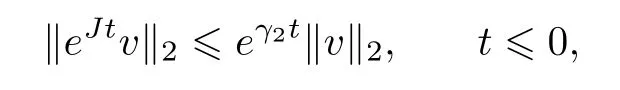

with a constant

γ

>

0 for all

v

∈

H

.

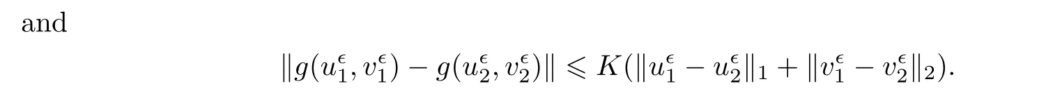
Hypothesis H2

(Lipschitz condition)Nonlinearities

f

and

g

are continuous and differentiable functions(

C

-smooth)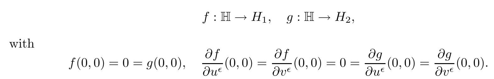

Hypothesis H3

(Gap condition)In the system,the term

K

(Lipschitz constant)of the functions

f

and

g

satis fies the bound

where

λ

is the first eigenvalue of the fractional Laplacian operator

A

.

Now we construct a random evolutionary system corresponding to the stochastic evolutionary system(3.1)–(3.2).For the achievement of this objective,we first set up the existence;after that we verify the uniqueness of the solution for equations(3.1)–(3.2)and for the Ornstein-Uhblenbeck equation.

Lemma 3.1

Let the

W

taking values in Hilbert space H be a two sided Wiener process.then,under hypotheses(H1)–(H3),system(3.1)–(3.2)possesses a unique mild solution.

Proof

We write system(3.1)–(3.2)in the following form:

is also an in finitesimal generator of the semigroup,which is strongly continuous.Therefore,the

W

taking values in Hilbert space H is a two sided Wiener process.Hence,by Theorem 7.2([15],p.188),system(3.1)–(3.2)possesses a unique mild solution.□

Lemma 3.2

The nonlocal stochastic equation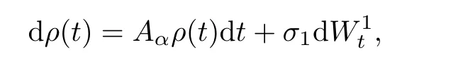

where

A

is the fractional Laplacian operator,has the solution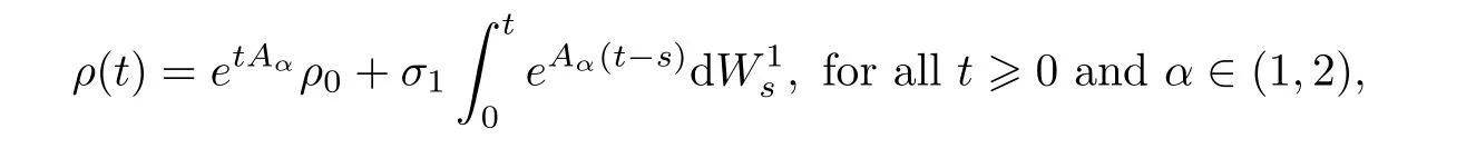

where

ρ

(0)=

ρ

is F-measurable.An equation being in

H

means that every term in the equation is in

H

.

Remark 3.3

([4])The above lemma does not hold for

α

∈(0

,

1].

Consider the stochastic evolutionary equations

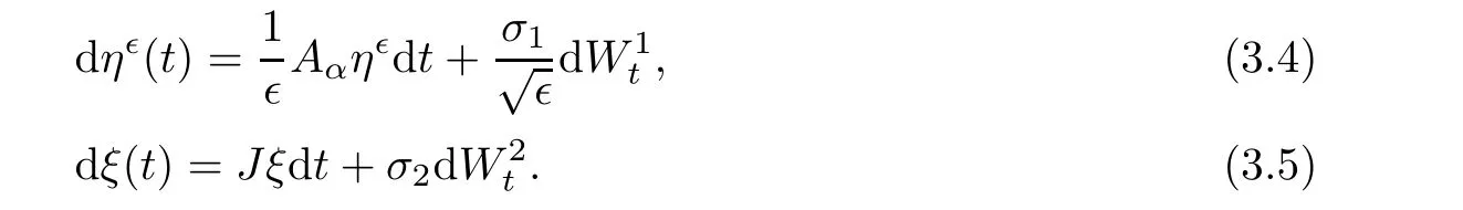
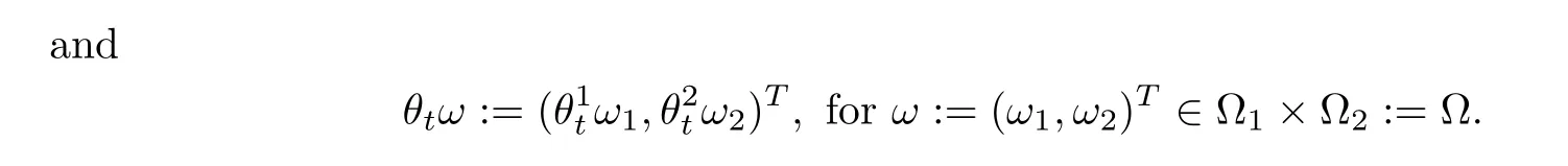
Introduce a random transformation

so that the original stochastic evolutionary system(3.1)–(3.2)is converted to a random evolutionary system as

The nonlinear functions

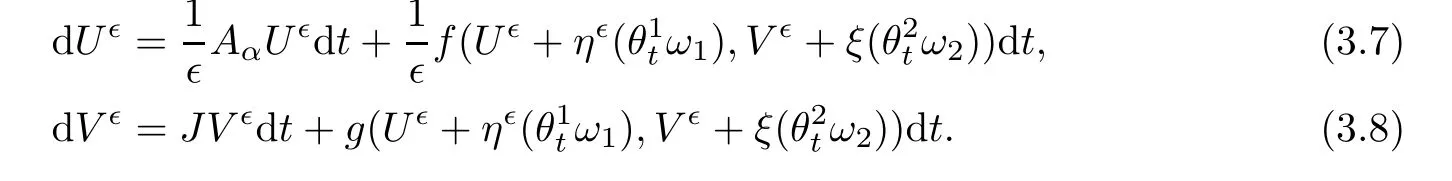
f

and

g

in(3.7)–(3.8)satisfy the same Lipschitz condition.Let

Z

(

t,ω,Z

)=(

U

(

t,ω,

(

U

,V

))

,V

(

t,ω,

(

U

,V

)))be the solution of(3.7)–(3.8)with initial value

Z

:=(

U

(0)

,V

(0))=(

U

,V

).By the classical theory for evolutionary equations[20],under the hypotheses(H1)–(H3),system(3.7)–(3.8)with initial data has a unique global solution for every

ω

=(

ω

,ω

)∈?=?×?,just like[10].

Hence,the solution mapping of random evolutionary system(3.7)–(3.8),

indicates a random dynamical system.Furthermore,

is the random system generated by the original stochastic system(3.1)–(3.2).

4 Slow Manifold

In this part,we construct the existence of the slow manifold and verify the exponential tracking property for the random evolutionary system(3.7)–(3.8).To study system(3.7)–(3.8),we construct the following Banach spaces in term of functions with a weighted geometrically sup norm[38]:for any

β

∈R,

with the norms

Similarly,we de fine

with the norms

For convenience,let

μ

be a number which satis fies

Now,for the achievement of our goal,the following Lemma from[10]is needed:

Lemma 4.1

Consider the so-called Lyapunov-Perron equation

for

V

∈

H

,where

U

(

s,ω

;

V

)and

V

(

s,ω

;

V

)are the solutions of system(3.7)–(3.8)with initial value

Z

=(

U

,V

)satisfying the form

Theorem 4.2

(Slow manifold)Suppose that(H1)–(H3)hold and that

?>

0 is small enough.Then random evolutionary system(3.7)–(3.8)possesses a Lipschitz random slow manifold

M

(

ω

)represented by a graph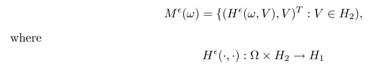

is a graph mapping with a Lipschitz constant satisfying

Remark 4.3

Since there is a relation between the solutions of stochastic evolutionary system(3.1)–(3.2)and random system(3.7)–(3.8),if system(3.1)–(3.2)satis fies the conditions described in Theorem 4.1,then it also possesses a Lipschitz random invariant manifold

Remark 4.4

If

f

and

g

are

C

,and the large spectrum gap condition mentioned in previous work[17]holds,then it can be proved in a fashion similar to[17]that the manifolds are

C

-smooth.

Proof of Theorem 4.1

To establish an invariant manifold corresponding to the random dynamical system(3.7)–(3.8),we first consider the integral equation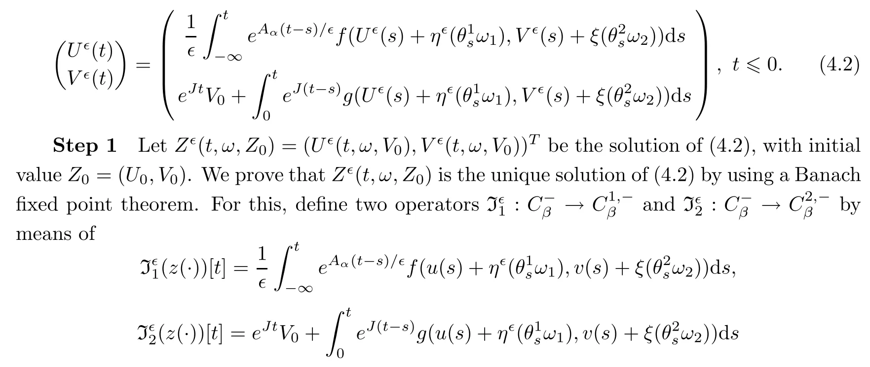

for

t

≤0.The Lyapunov-Perron trans form Iis

Hence,combining this with the de finition of I,we obtain that

where

C

,i

=1

,

2

,

3

,

4 are constants and

Furthermore,to show that the map Iis contractive,we take

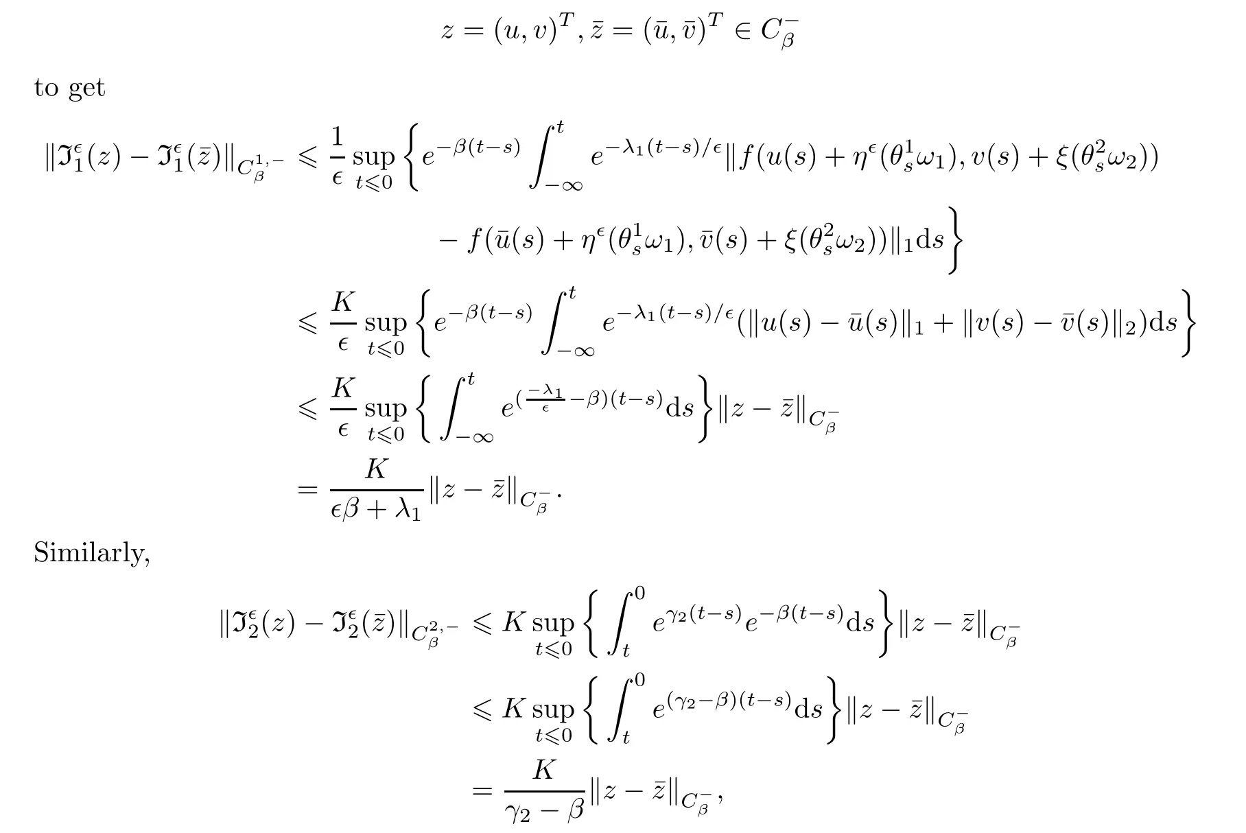
which implies that

Therefore,there is a small enough parameter

?

→0 such that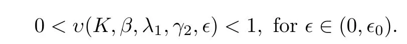

Furthermore,

Thus,we obtain the upperbound

for all

ω

∈?

,V

,V

∈

H

.

Step 2

With help of the unique solution described in Step 1,we construct the mapping

H

as follows:

Then,owing to(4.3),we obtain upperbound

for all

V

,V

∈

H

and

ω

∈?.This implies that

for all

V

,V

∈

H

and

ω

∈?.Then,by Lemma 4.3,it follows that

Step 3

In this step,to prove that

M

(

ω

)is a random set,we prove that,for any

z

=(

u,v

)∈H=

H

×

H

,

is measurable(Theorem III.9 in Casting and Valadier[9],p.67).Let separable space H have a countable dense set,say,H.Then the right hand side of(4.5)is equal to

Step 4

Now it only remains to show that the random set

M

(

ω

)is positively invariant;that is,we prove that for each

Z

=(

U

,V

)∈

M

(

ω

)

,Z

(

s,ω,Z

)∈

M

(

θ

ω

)for all

s

≥0

.

Finally,for every fixed

s

≥0

,

we may observe that

Z

(

t

+

s,ω,Z

)is a solution of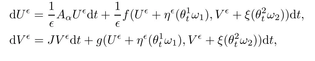

with initial data

Z

(0)=(

U

(0)

,V

(0))=

Z

(

s,ω,Z

).

Here Cand Care positive constants.

Remark 4.6

By the relationship between the solutions of(3.1)–(3.2)and(3.7)–(3.8),if system(3.7)–(3.8)has an exponential tracking manifold,so does the original stochastic system(3.1)–(3.2).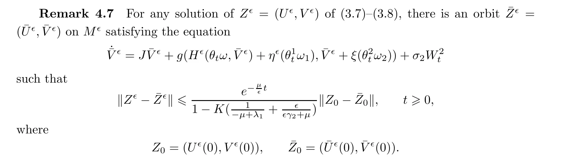

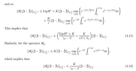
From Theorem 4.1,we know that

Now,we get the upperbound by combining(4.11)and(4.12):

so,by(4.1),there is a sufficiently small constant?

?

>

0 such that

Furthermore,

which means that

Since the exponential tracking property of

M

(

ω

)is obtained,this completes the proof.

With the help of Remarks 4.4 and 4.5,we get a reduced system based on a slow manifold for the original fast-slow stochastic evolutionary system(3.1)–(3.2),stated as Theorem 4.3.

5 Parameter Estimation on Random Slow Manifold

Assume that original slow equation(3.2)has an unknown parameter

d

∈R and that we know that its range is denoted by∧,which is a close interval.In other words,the nonlocal fast-slow system(3.1)–(3.2)becomes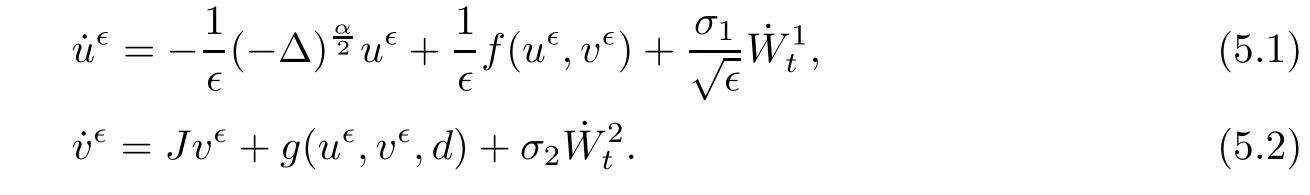

In this section,we establish a parameter estimation method for a nonlocal stochastic system by using only the observations on the slow component,and we do so with on error estimation.

5.1 Parameter estimation based on reduced slow system

Importance

The slow system has a lower dimension than the original nonlocal stochastic system.In terms of computational cost our method offers the bene fit of using observations only on slow components;compared to fast components,it is often much more reliable to observe slow components[33].

We estimate the system parameter

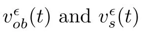
d

in(5.1)–(5.2)using the reduced slow system

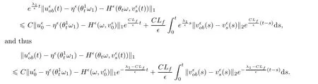
and now,by Cauchy-Schwarz inequality,

By using a variation of constants formula,we obtain that

and then

By using a variation of constants formula,we obtain that

By Gronwall’s inequality,we obtain

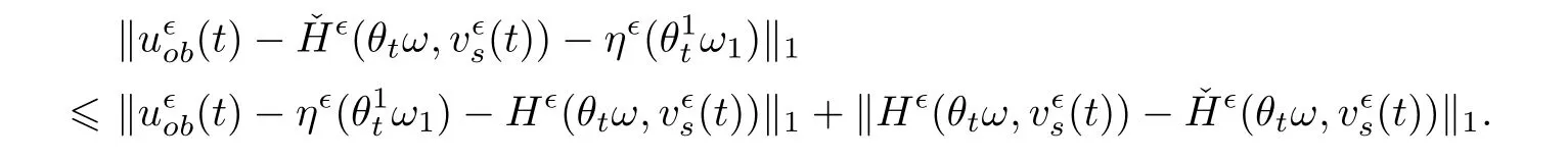
Now,we conclude by exchanging the order of integrals as follow:

Thus,by Cauchy-Schwartz inequality,

Consider the integral term,which is on the left hand side of(5.8),and set

then the approximate reduced slow system is

for the estimation.Note that

6 Examples

To observe the results regarding the existence of slow manifolds which were obtained in the previous section,let us look at a few examples.

Example 6.1

Take a system with

γ

=0,system(6.1)–(6.2)has a random manifold

M

(

ω

)={(

H

(

ω,V

)

,V

):

V

∈

H

}with an exponential tracking property if

and

?>

0 is sufficiently small.

The preceding system may be a model of certain biological processes[14,21,30].

In Example 2,we illustrate our analytical results via numerical simulation.

Example 6.2

Take a fast-slow stochastic system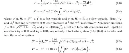

Random dynamical system(6.5)–(6.6)has a slow invariant manifold,for sufficiently small

?>

0,such that

Based on[4,32],we plot the graph of the slow manifolds approximately to order O(

?

).Let

t

=

τ?

and

with initial value

U

(0)=

H

(

ω,V

)=

H

+

?H

+

...,

and

V

(0)=

V

.

Then,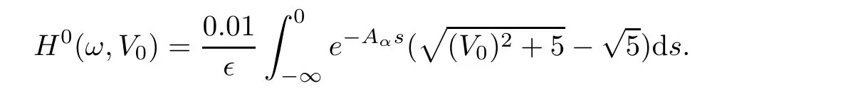

Finally,the approximate reduced slow system is

We conducted the numerical simulations to illustrate the slow manifold,the exponential attracting property and the parameter estimation based on the slow system in Figures 1–4.

Figure 1 Random slow manifold for different samples for Example 2

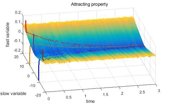
Figure 2 Exponential tracking property for Example 2:σ1=σ2=0.1,α=1.2 and?=0.01.It shows that all solutions are attracted towards the evolutionary slow manifold.

Figure 3 Parameter estimation for the original fast-slow nonlocal stochastic system.For Example 2:σ1=σ2=0.1,α=1.2 and?=0.01.The estimation value is 5.0000 with error 9.7656e-05 and objective function value is 2.9724e-31 after 19 number of iterations and 3980.714622 seconds

Figure 4 Parameter estimation for the reduced slow system for Example 2:σ1=σ2=0.1,α=1.2 and?=0.01.The estimation value is 5.0573 with error 0.0573 and objective function value is 1.0979e-07 after 33 number of iterations and 645.638133 seconds

Each curve stands for a sample:

σ

=

σ

=0

.

1

,α

=1

.

2 and

?

=0

.

01.

From Figures 3 and 4,we can conclude that the error for the simulation of parameter estimation based on the reduced system is nearly equal to the error based on the original system.However,simulation of parameter estimation based on the reduced system needs much less time than the original system,so it is acceptable.