PHASE PORTRAITS OF THE LESLIE-GOWER SYSTEM*

Departament de Matemàtiques,Universitat Autònoma de Barcelona,08193 Bellaterra,Barcelona,Catalonia,Spain

E-mail: jllibre@mat.uab.cat

Claudia VALLS?

Departamento de Matemática,Instituto Superior Técnico,Universidade de Lisboa,Av.Rovisco Pais 1049–001,Lisboa,Portugal

E-mail: cvalls@math.tecnico.ulisboa.pt

Abstract In this paper we characterize the phase portraits of the Leslie-Gower model for competition among species.We give the complete description of their phase portraits in the Poincaré disc (i.e.,in the compactification of R2 adding the circle S1 of the infinity) modulo topological equivalence.It is well-known that the equilibrium point of the Leslie-Gower model in the interior of the positive quadrant is a global attractor in this open quadrant,and in this paper we characterize where the orbits attracted by this equilibrium born.

Key words predator-prey models;Leslie–Gower system;Poincaré compactification;global phase portraits

1 Introduction and Statement of the Main Results

The dynamical relations between predators and prey is one of the fundamental objects of study in population dynamics.This is mainly due to the fact that to its big number of applications [3] and because it allows a better understanding of the behavior of food chains or trophic networks (see for instance [14,24]).

The first predator-prey model was proposed by the italian mathematician Vito Volterra[1,2] in its celebrate publish monograph in 1926 [25] where he described the model as a nonlinear system of ordinary differential equations.This model coincided with a bidimensional model for biochemic interactions proposed earlier by the american physicist Alfred J.Lotka and this is the main reason why these type of models are called Lotka-Volterra models [2,14,15,24].The main feature of this model is that the unique positive equilibrium point is a center and all the orbits are closed concentric orbits around the equilibrium point.This implies that the population sizes of the predators and prey oscillate permanently around this point for any initial condition.This behavior of the solutions of the system was early questioned because this is not what happens in nature.

After Volterra’s work,there were many attempts to solve the objections of Volterra’s model.One of this attempts was Leslie–Gower model [9] whose main feature is that the predator growth equation is of logistic type (see [1]) and so it considers implicitly that there exists competition or self-interference between the predators.The Leslie–Gower model has been studied from many points of view,see for instance the recent papers [5–8,10–12,19–23,26–33].As far as we know there are no results concerning the characterization of its global dynamics taking into account the orbits which come or scape at infinity.Thus,in this work we will study the global phase portraits of this model in the Poincaré disc.

The Leslie–Gower model is described by the differential equations of the form

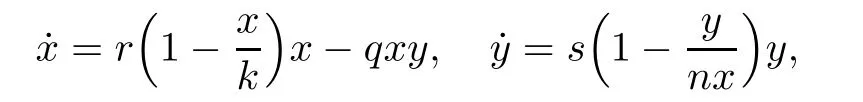
where the dot means derivative with respect to the timetand all the parametersr,k,q,s,nare positive and have the following meaning:ris the intrinsic rate of growth prey,kis the environmental bearing capacity for prey,qis the maximum consumption rate (maximum quantity of necessary prey that can be consumed for each predator in each unity of time),sis the intrinsic rate of growth predators andnis the quantity of prey with food for the predators.

This system is not defined in (0,0).Making the reparameterization dτ=nxdt,we obtain the equivalent system

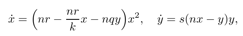
where the dot denotes derivative with respect to the new independent variableτ.Now doing the change (x,y,τ) →(X,Y,T) given by

where the dot denotes derivative in the new timeTandA=knq/r,B=s/rbeingA,B ＞0 and we have renamed the variables (X,Y) again as (x,y).Note that system (1.2) is a continuous extension of the original Leslie–Gower system.

In fact we shall present the distinct global phase portraits of the Leslie–Gower system when its parametersA,Bvaries in R+in the Poincaré disc.In this way we can describe the dynamics of their orbits which come or go to the infinity of R2.For doing this we will use the Poincaré compactification.

Roughly speaking the Poincaré compactification of a polynomial differential system consists in extending this system to an analytic system on a closed disc D2of radius one,whose interior is identified with R2and its boundary,the circle S1,plays the role of the infinity.This closed disc is called the Poincaré disc,because the technique for doing such an extension is due to Poincaré.For details on this compactification see [4,chapter 5] or the summary presented in Subsection 2.1.

Theorem 1.1The phase portraits of system (1.2) in the Poincaré disc are totpologically equivalent to one of the 2 phase portraits presented in Figure 1.

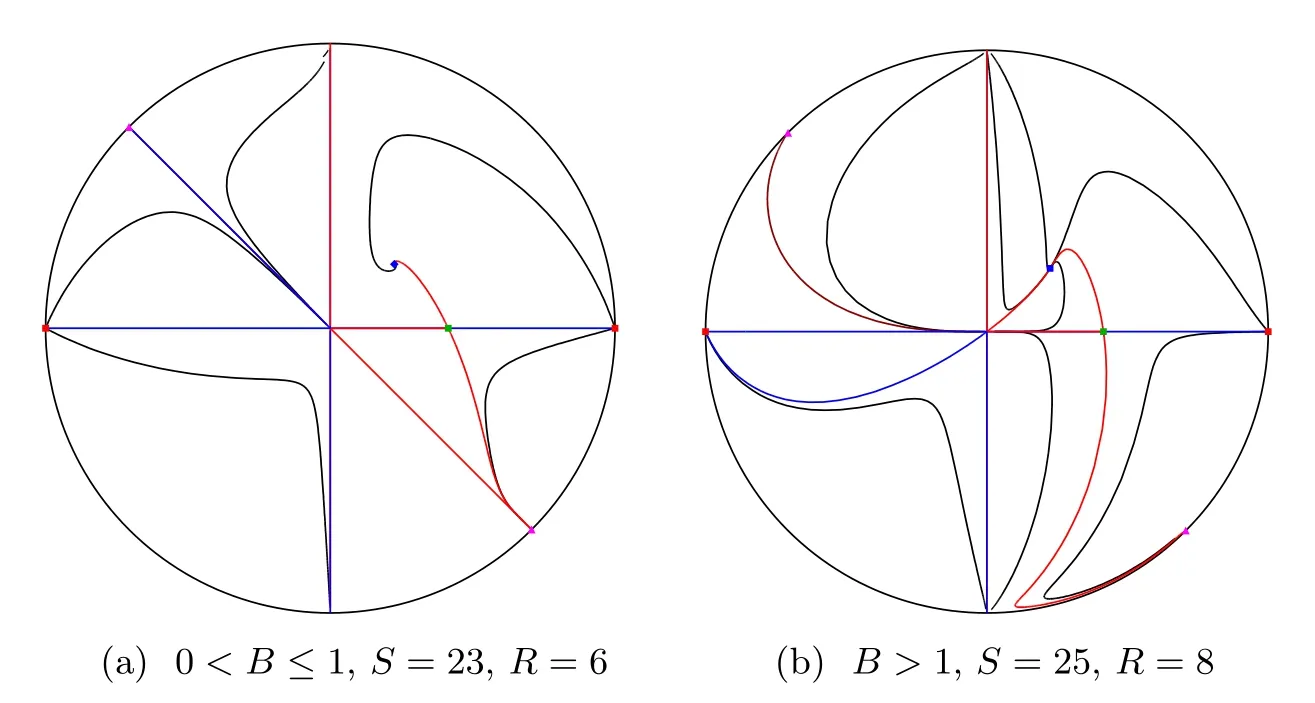
Figure 1 Phase portraits of system (1.2) on the Poincaré disc

The proof of Theorem 1.1 is given in Section 3.

In Figure 1Sdenotes the number of separatrices andRdenotes the number of canonical regions.See for more details in Subsection 2.1.

In Subsection 3.2 we will show that system (1.2) has three equilibria,pjforj=1,2,3.

In the next corollary we provide new information from the ecological Leslie–Gower predatorprey model.It is well-known that the equilibrium pointp3in the interior of the positive quadrant is a global attractor in this open quadrant,but it is was unknown where the orbits attracted byp3born.

Corollary 1.2The following two staements hold.

(a) If the parameter 0＜B≤1,then all the orbits of the Leslie–Gower system (1.1)attracted byp3come from the endpoint of the positivex-half-axis,except one orbit coming from the poinfp2.

(b) If the parameterB ＞1,then all the orbits of the Leslie–Gower system (1.1) attracted byp3come from either the endpoint of the positivex-half-axis,or from the endpoint of the positivey-half-axis,or from the origin,except one orbit coming from the pointp2.

The proof of Corollary 2 follows immediately from the phase portraits of Figure 1.

2 Preliminary Results

2.1 Poincaré compactification

In order to classify the global dynamics of a polynomial differential system the first crucial step is to characterize their finite and infinite equilibrium points in the Poincaré compactification[18].The second main step for determining the global dynamics in the Poincaré disc of a polynomial differential system is the characterization of their separatrices.For the polynomial differential systems in the Poincaré disc it is known that the separatrices are the infinite orbits,the finite equilibrium points,the separatrices of the hyperbolic sectors of the finite and infinite equilibrium points,and the limit cycles.If Σ denotes the set of all separatrices in the Poincaré disc D2,Σ is a closed set and the components of D2 Σ are called the canonical regions.We denote by S and R the number of separatrices and canonical regions,respectively.

We consider the set of all polynomial vector fields in R2of the form

wherePandQare real polynomials in the variablesxandyof degreesd1andd2,respectively.Taked=max{d1,d2}.

Denote byTpS2be the tangent space to the 2-dimensional sphere

at the pointp.Assume thatXis defined in the planeT(0,0,1)S2=R2.Consider the central projectionf:T(0,0,1)S2→S2.This map defines two copies ofX,one in the open northern hemisphere and the other in the open southern hemisphere.Denote byX′the vector fieldDf°Xdefined onS2except on its equator S1={s∈S2:s3=0}.Clearly S1is identified to the infinity of R2.IfXis a planar polynomial vector field of degreed,thenp(X) is the only analytic extension of.The vector fieldp(X) is called the Poincaré compactification of the vector fieldX,for more details see [4,chapter 5].

On the Poincaré sphere S2we use the following six local charts,which are given byUi={s ∈S2:si＞0} andVi={s ∈S2:si＜0},fori=1,2,3,with the corresponding diffeomorphisms

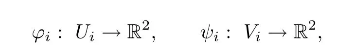
defined byφi(s)=-ψi(s)=(sm/si,sn/si)=(u,v) form ＜nandm,n≠i.Thus (u,v) will play different roles in the distinct local charts.The expressions of the vector fieldp(X) are

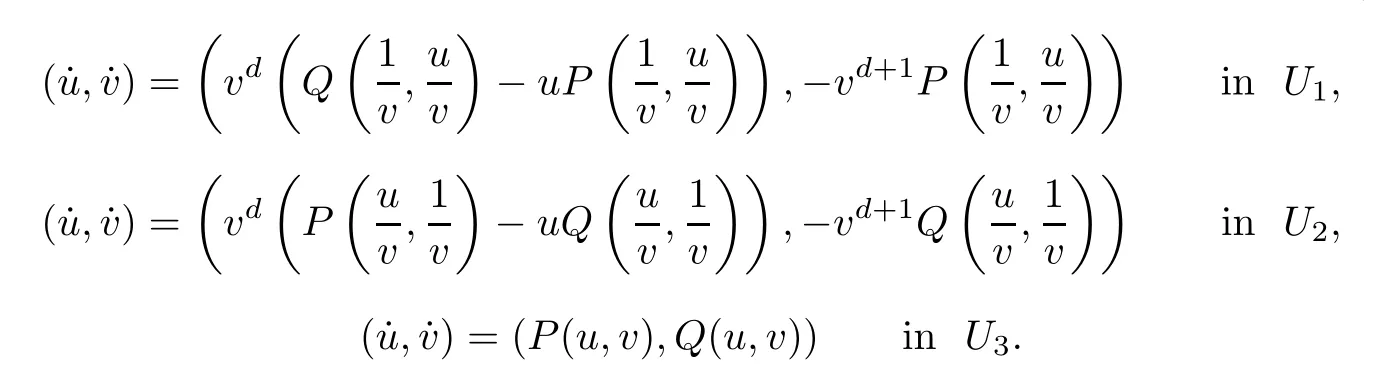
We note that the expressions of the vector fieldp(X) in the local chart (Vi,ψi) is equal to the expression in the local chart (Ui,φi) multiplied by (-1)d-1fori=1,2,3.

The orthogonal projection underπ(y1,y2,y3)=(y1,y2) of the closed northern hemisphere of S2onto the planes3=0 is a closed disc D2of radius one centered at the origin of coordinates called the Poincaré disc.Since a copy of the vector fieldXon the plane R2is in the open northern hemisphere of S2,the interior of the Poincaré disc D2is identified with R2and the boundary of D2,the equator S1of S2,is identified with the infinity of R2.Consequently the phase portrait of the vector fieldXextended to the infinity corresponds to the projection of the phase portrait of the vector fieldp(X) on the Poincaré disc D2.

The equilibrium points ofp(X) in the Poincaré disc lying on S1are the infinite equilibrium points of the corresponding vector fieldX.The equilibrium points ofp(X) in the interior of the Poincardisc,i.e.,on S2 S1,are the finite equilibrium points.We note that in the local chartsU1,U2,V1andV2the infinite equilibrium points have their coordinatev=0.

For a polynomial vector field (2.1) ifs∈S1is an infinite equilibrium point,then -s∈S1is another infinite equilibrium point.Thus the number of infinite equilibrium points is even and the local phase portrait of one is that of the other multiplied by (-1)d+1.

2.2 Separatrix skeleton

Given a flow (D2,φ) by the separatrix skeleton we mean the union of all the separatries of the flow together with one orbit from each one of the canonical regions.LetC1andC2be the separatrix skeletons of the flows (D2,φ1) and (D2,φ2) respectively.We say thatC1andC2are topologically equivalent if there exists a homeomorphismh: D2→D2which sends orbits to orbits preserving or reversing the direction of all orbits.From Markus [13],Neumann [16] and Peixoto [17] it follows the next theorem which shows that is enough to describe the separatrix skeleton in order to determine the topological equivalence class of a differential system in the Poincaré disc D2.

Theorem 2.1(Markus–Neumann–Peixoto theorem) Assume that (D2,φ1) and (D2,φ2)are two continuous flows with only isolated equilibrium points.Then these flows are topologically equivalent if and only if their separatrix skeletons are equivalent.

3 Proof of Theorem 1.1

We will state and prove several auxiliary results.As pointed out in the introduction we will work with system (1.2) instead of the original Leslie–Gower system.

3.1 Limit cycles

To state and prove the first of our results we recall the Bendixson–Dulac theorem: consider a planar continuously differentiable system

defined in some open simply connected subsetU?R2and setX=(P,Q).Assume that there exists a continuously differentiable functionF:U→R such that

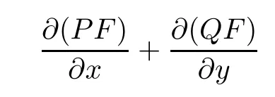
does not change sign and vanishes only on a set of zero Lebesgue measure.Then system (3.1)has no periodic orbits contained inU.

Proposition 3.1System (1.2) has no limit cycles.

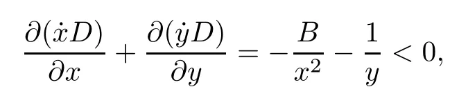
ProofBy uniqueness of solutions it is clear that if system (1.2) has periodic orbits they do not intersect the coordinate axes.By making the change of variablesx→±x,y→±y,if necessary,we can restrict our study to the first quadrant

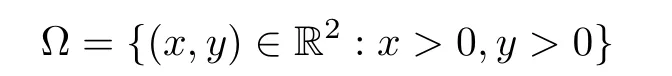
and prove that system (1.2) has no periodic orbits on it.We consider the functionD: Ω →R,given byD(x,y)=1/(x2y).Note that it is continuously differentiable in Ω.Moreover,becauseB ＞0.Now we can apply the Bendixson-Dulac theorem and since Ω is simply connected the system has no limit cycles.This concludes the proof of the proposition. □

3.2 Finite equilibrium points

Now we study the finite equilibrium points of system (1.2).We introduce the notation

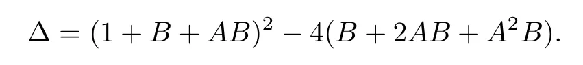
Proposition 3.2System (1.2) has three singular pointsp1=(0,0),p2=(1,0) andp3=(1,1)/(A+1).The singularp1is formed by two hyperbolic and two parabolic sectors,the singular pointp2is a saddle and the singular pointp3is a stable node if Δ ≥0 and a stable focus if Δ＜0.

In the proof of the proposition we provide the explicit position of the hyperbolic and parabolic sectors forp1in function of the values of the parameterB.

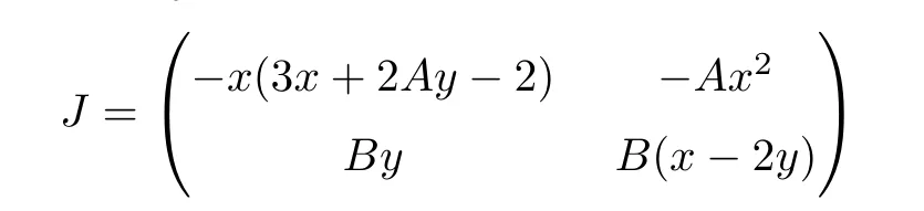
ProofIt is clear that the singular points arep1=(0,0),p2=(1,0) andp3=(1,1)/(A+1).The Jacobian matrix of the system is

The eigenvalues of the Jacobian matrix at the singular pointp2are -1,B.SinceB ＞0,the singular pointp2is a hyperbolic saddle.

The Jacobian matrix of the singular pointp1isand sop1is linearly zero.To obtain the local behavior of this point we will use the blow-up technique.To do so,letz=y/xand we get the equation

Rescaling by the independent variable (the time) bys=xTwe obtain the system

where the dot means derivative in the new variables.

The Jacobian matrix evaluated at (0,0) has the eigenvalues 1 andB-1.Therefore the point (0,0) is a saddle if and only ifB ＜1,an unstable node if and only ifB ＞1 and a saddle-node if and only ifB=1.Moreover,the Jacobian matrix evaluated at (0,(B-1)/B)has the eigenvalues 1 and -(B-1).Therefore the point (0,(B-1)/B) is a saddle if and only ifB ＞1,an unstable node if and only ifB ＜1 and a saddle-node if and only ifB=1.

Doing the blow-down process we obtain that ifB∈(0,1] then the local phase portrait at the origin is the following: in the first quadrant (the positive quadrant) there is a hyperbolic sector and in the second quadrant there is an attractor parabolic sector.The boundary of this sector is on the negativex-half axis and on the positivey-half axis and all the other orbits of this parabolic sector arrive to the origin with slope (B-1)/B.In the third quadrant we have another hyperbolic sector and,finally in the fourth quadrant we have a repeller parabolic sector.The boundary of this parabolic sector is again thexandyaxes and all the other orbits of this sector exit from the origin with slope (B-1)/B.Furthermore,whenB ＞1 we get that topologically the local phase portrait of the origin is the same as the one forB∈(0,1],but the separatrix of the sector which was on the positivex-half axis now is inside the first quadrant with slope (B-1)/B,and the separatrix of the hyperbolic sector which was contained in the third quadrant now is in the interior of this quadrant with slope (B-1)/B.

The eigenvalues of the Jacobian matrix at the singular pointp3is are

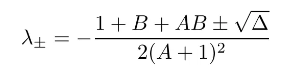
SinceA,B ＞0 we have thatand soλ±＜0.Hence,the pointp3is locally a stable node if Δ ≥0 and is locally a stable focus if Δ＜0.This concludes the proof of the proposition. □

3.3 Infinite equilibrium points

Proposition 3.3System (1.2) has three pairs of infinite equilibrium points: the origin of the local chartU1(denoted byq1) and its diametrally opposite point,q2=(-1/A,0) (and its diametrally opposite point) and the origin of the local chartU2(denoted byq3) and its diametrally opposite point.The infinite equilibrium pointq1is an unstable node,q2is a saddle-node andq3is formed by two hyperbolic and two parabolic sectors.

In the proof of the proposition we provide the explicit position of the hyperbolic and parabolic sectors forq3.

ProofSystem (1.2) on the local chartU1becomes

The equilibrium points onv=0 are the solutions ofu(1 +Au)=0 and so we have two equilibrium pointsq1=(0,0) andq2=(-1/A,0).

Computing the eigenvalues of the Jacobian matrix atq1we get that they are 1,1 and soq1is an unstable node.

Computing the eigenvalues of the Jacobian matrix atq2we get that they are (0,-1) so the pointq2is semi-hyperbolic.Using [4,Theorem 2.19] we conclude thatq2is a saddle-node.Indeed,translating the pointq2to the origin and making a rescaling of times=-τwe get the new system

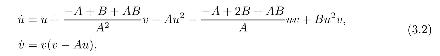
where the dot means derivative in the new times.In order to apply [4,Theorem 2.19] we must pass the linear part of system (3.2) to its Jordan normal form.This is made doing the linear change of variables

In these new variables system (3.2) becomes

Applying [4,Theorem 2.19] we get thatq2is a saddle-node having the nodal sector in the local chartU1and the two hyperbolic sectors in the local chartV1.

Now we compute system (1.2) on the local chartU2and we obtain

We only need to study the origin of the local chartU2which we denote byq3.Note that the Jacobian matrix evaluated atq3isand so the point is linearly zero.We need to apply the blow-up technique.To do so,letw=v/uand we get the equation

Reescaling by the independent variable (the time) bys=uτwe obtain the system

where the dot means derivative in the new variables.The unique equilibrium point over the straight lineu=0 is the origin which is a saddle because their eigenvalues are ±A.Doing the blow-down process,going back through the changes of variables and taking into account how is the flow on the invariant axes,we obtain that the origin ofU2is formed by two hyperbolic sectors and two parabolic sectors.More precisely,in the first quadrant in the plane (u,v) we have a hyperbolic sector,the separatrices are on the axes.In the second quadrant we have a repeller parabolic sector whose separatrices are on the axes,in the third quadrant we have hyperbolic sector and,finally,in the fourth quadrant we have an attractor parabolic sector.□

3.4 Global phase portraits

From Subsection 2.2 and Proposition 3.1 in order to prove Theorem 1 we only need to determine the behaviour of the separatrices of the hyperbolic sectors of the finite and infinite singular points,i.e.where they born and where they die.Doing so we will have all the separatrix skeleton adding one orbit in each canonical region,and consequently we will have the global phase portraits of system (1.2).But taking into account the two invariant straight lines and the local phase portraits at all the finite and infinite singular points,the place where born and die all the separatrices of the hyperbolic sectors is determined in a unique way for every one of the two cases in function of the parameterBeither if 0＜B≤1 or ifB ＞1.In this way we obtain the 2 phase portraits in the Poincaré disc of Figure 1.This completes the proof of Theorem 1.