GLOBAL WELL-POSEDNESS FOR THE FULL COMPRESSIBLE NAVIER-STOKES EQUATIONS*

School of Mathematics and Computer Sciences,Gannan Normal University,Ganzhou 341000,China Department of Mathematics,Sun Yat-sen University,Guangzhou 510275,China

E-mail: lijl29@mail2.sysu.edu.cn

Zhaoyang YIN (殷朝陽)

Department of Mathematics,Sun Yat-sen University,Guangzhou 510275,China Faculty of Information Technology,Macau University of Science and Technology,Macau,China

E-mail: mcsyzy@mail.sysu.edu.cn

Xiaoping ZHAI (翟小平)?

Department of Mathematics,Guangdong University of Technology,Guangzhou 510520,China School of Mathematics and Statistics,Shenzhen University,Shenzhen 518060,China

E-mail: pingxiaozhai@163.com

Abstract We are concerned with the Cauchy problem regarding the full compressible Navier-Stokes equations in Rd (d=2,3).By exploiting the intrinsic structure of the equations and using harmonic analysis tools (especially the Littlewood-Paley theory),we prove the global solutions to this system with small initial data restricted in the Sobolev spaces.Moreover,the initial temperature may vanish at infinity.

Key words compressible Navier-Stokes equations;global well-posedness;Friedrich’s method;compactness arguments

1 Introduction and the Main Result

The full compressible Navier-Stokes equations can be written in the sense of Eulerian coordinates in Rdas follows:

Hereρ(t,x),u(t,x)=(u1,u2,· · ·,ud)(t,x) andθ(t,x) stand for the density,the velocity and the temperature of the fluid,respectively.In addition

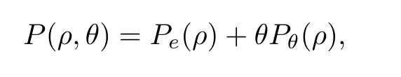
wherePe(ρ) andθPθ(ρ) denote elastic pressure and thermal pressure,respectively.Such pressure laws cover the cases of ideal fluids (for whichPe(ρ)=0 andPθ(ρ)=Rρfor a universal constantR ＞0),of barotropic fluids (Pθ(ρ)=0),and of Van der Waals fluids (Pe=-αρ2,Pθ=βρ/(δ-ρ) withα,β,δ ＞0).The viscous stress tensor S=μ(ρ)(?u+(?u)T) characterizes the measure of resistance of fluid to flow.,andcv(θ) represents the specific heat at a constant volume.The heat conductionqis given byq=-κ(θ)?θ(see,e.g.,the introduction of [14]).

This model has been studied by many mathematicians and much progress has been made in recent years,due to the significance of the physical background.There has been a great deal of work about the existence,uniqueness,regularity and asymptotic behavior of the solutions (see[6,8,10,14,15,18,20–22,28–30,37,38,40]).However,because of the stronger nonlinearity in(1.1) compared with the Navier-Stokes equations for isentropic flow (no temperature equation),many known mathematical results have focused only on the absence of a vacuum (a vacuum means thatρ=0).The local existence and uniqueness of smooth solutions of (1.1) were proved by Nash [32] for smooth initial data without a vacuum.Itaya [24] considered the Cauchy problem of the Navier-Stokes equations in R3with a heat-conducting fluid,and obtained the local classical solutions in Hlder spaces.The same result was obtained by Tani [33] for IBVP with infρ0＞0.Later on,Matsumura and Nishida [30] proved the global well-posedness for smooth data close to equilibrium;see also [27] for one dimension.Regarding the existence,and the asymptotic behavior of the weak solutions of the full compressible Navier-Stokes equations with infρ0＞0,please refer,for instance,to [25],and to [26] for the existence of weak solutions in 1D and for the existence of spherically symmetric weak solutions in Rd(d=2,3),respectively.Refer to [19] for the existence of spherically and cylindrically symmetric weak solutions in R3,and to [15] for the existence of variational solutions in a bounded domain in Rd(d=2,3).

For results in the presence of a vacuum,Feireisl [14] got the existence of the so-called variational solutions in Rd(d≥2).The temperature equation in [14] is satisfied only as an inequality in the sense of distributions.In order that the equations are satisfied as equalities in the sense of distributions,Bresch and Desjardins [2] proposed some different assumptions from[14],and obtained the existence of global weak solutions to the full compressible Navier-Stokes equations with large initial data in T3or R3.Huang,Li and Xin [23] established the global existence and uniqueness of classical solutions to the three-dimensional isentropic compressible Navier-Stokes system with smooth initial data;these are of small energy but possibly large oscillations where the initial density is allowed to vanish.Wen and Zhu [35] obtained the global existence of spherically and cylindrically symmetric classical and strong solutions of the full compressible Navier-Stokes equations in R3.The result in [35] allows the initial data to be large and for the initial density to vanish.We also emphasize some blowup criteria from [20–22](see also the references therein).The reader may refer to [6,18,28,29,35,36,40] for more recent advances on the subject.

Let us also recall that in the barotropic case (that is,θ=0 in (1.1)),the critical Besov regularity was first considered by Danchin [9] in anL2type framework.The author obtained a global solution for small perturbations of a stable constant statewith ˉρ ＞0.Since then,there have been a number of refinements regarding admissible exponents for the global existence (see[3,5,7,17,39] and the references therein).For the non-isentropic compressible Navier-Stokes equations (1.1),Chikami and Danchin [8] and Danchin [10] considered the local wellposedness problem.Global small solutions in a criticalLpBesov framework were obtained,respectively,by Danchin [11] forp=2,and Danchin and He [13] for more generalp.It should be mentioned that the critical Besov space used in [8] and [13] seems to be the largest one in which the system (1.1)is well-posed.Indeed,Chen et al.[6] proved the ill-posedness of (1.1) inforp ＞3.Finally,we mention [18] the most recent result about the global-in-time stability of large solutions for the full Navier-Stokes-Fourier system in R3,as well as the work [40],on the convergence to equilibruim for the full Navier-Stokes-Fourier system in the bounded domain.

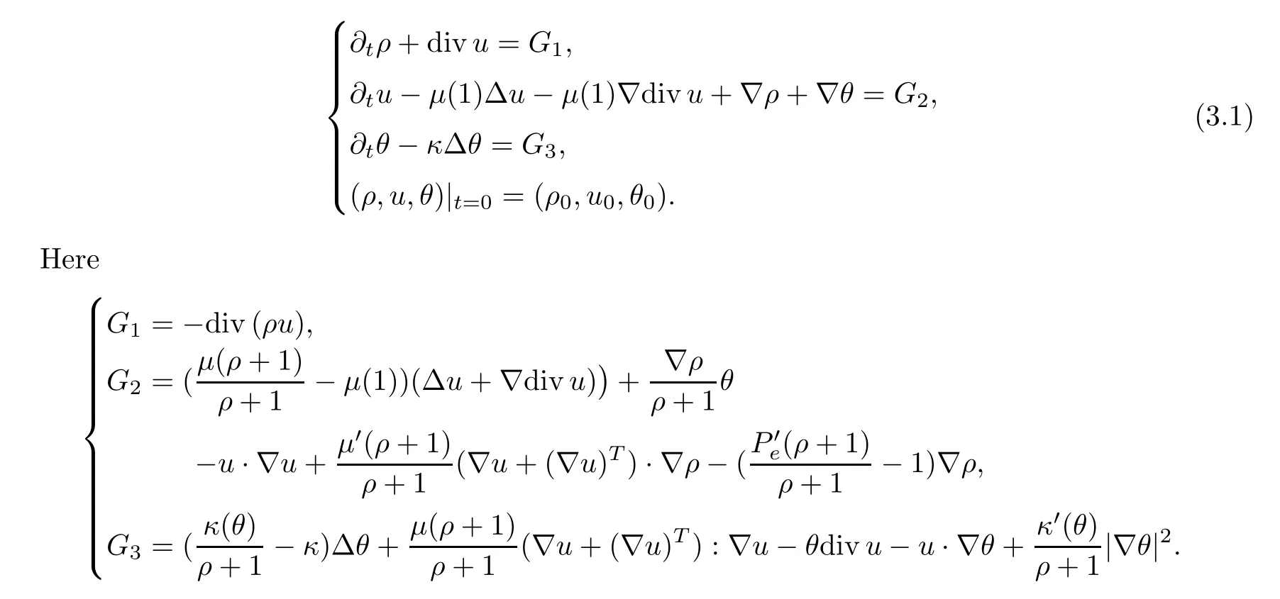
In the present paper,we will consider the Cauchy problem of (1.1) in Rd,d=2,3.We assume thatcv=1,P(ρ,θ)=Pe(ρ) +Rρθ,q=-κ(θ)?θ,Pe(ρ),κ(θ),μ(ρ) are smooth functions aboutρ,θ.Then the system (1.1) becomes

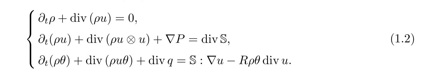
Due to the term divq=div (κ(θ)?θ)=κ(θ)Δθ+κ′(θ)|?θ|2,obviously,system (1.2) has no scaling invariance compared with the compressible Navier-Stokes equations with constant viscosities.

and with initial data

For notational simplicity,we assume that=1,R=1,(1)=1,μ(1)＞0 andκ(0)=κ ＞0.

Substitutingρwithρ+1,we reduce system (1.2) to the equations

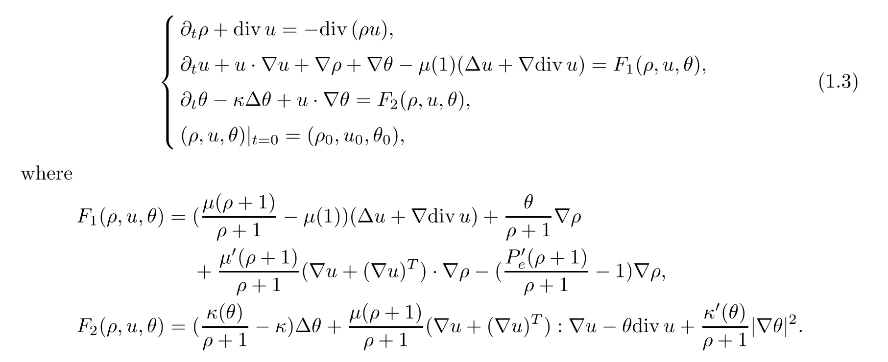
When solving (1.3),the main difficulty is that the system is only partially parabolic,owing to the mass conservation equation which is of hyperbolic type.This precludes any attempt to use the Banach fixed point theorem in a suitable space.As a matter of fact,global existence for small initial data may be proved through a suitable norm uniform bound estimate scheme and compactness methods.In this paper,we first use the Littlewood-Paley decomposition theory in Sobolev spaces to establish an energy estimate.Then we apply the classical Friedrich’s regularization method to build global approximate solutions and prove the existence of a solution by compactness arguments for the small initial data.Moreover,we can obtain that the solution to the system (1.3) is unique.

The main theorem of this paper reads as follows.

Theorem 1.1Letd=2,3 ands ＞For anyρ0∈Hs(Rd),u0∈Hs(Rd),θ0∈Hs(Rd),there exists a small constantη ＞0 such that

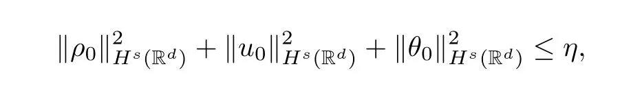
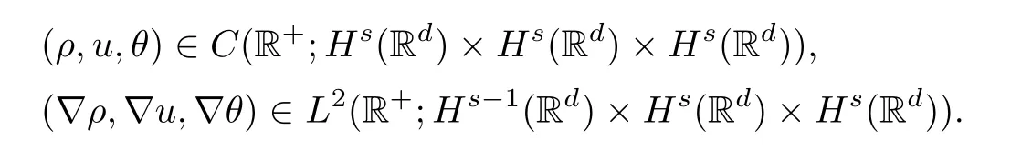
so the system (1.3) has a unique global solution (ρ,u,θ) satisfying

Remark 1.2Compared with the classical result by Matsumura and Nishida in [30],the regularity index of the initial data is lower,moreover,the temperature of the fluid cannot be near nonzero equilibrium here.

Remark 1.3It should be mentioned that our result covers the case of the ideal gasesP(ρ,θ)=Rρθ.

The rest of this paper is organized as follows: in Section 2,we recall the Littlewood-Paley theory and give some properties of inhomogeneous Sobolev spaces.In Section 3,we deduce a priori estimates of solutions to system (1.3).In Section 4,we prove the global existence and uniqueness of the solution to the system (1.3) by Fredrich’s method for the small initial data.

NotationsIn what follows,we denote by (·,·) theL2scalar product.Given a Banach spaceX,we denote its norm by ‖·‖X.The symbolA?Bdenotes that there exists a constantc ＞0 independent ofAandBsuch thatA≤cB.The symbolA≈BrepresentsA?BandB?A.

2 The Littlewood-Palely Theory

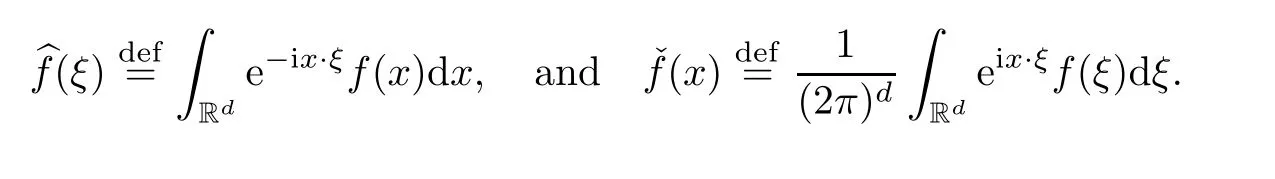
In this section,we are going to recall the dyadic partition of unity in the Fourier variable,the so-called Littlewood-Paley theory,and the definition of Besov spaces.Part of the material presented here can be found in [1].Let S(Rd) be the Schwartz class of rapidly decreasing functions.For givenf∈S(Rd),the Fourier transformand its inverse Fourier transformare defined,respectively,by

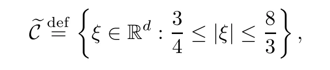
Letφ∈S(Rd) with values in [0,1] such thatφis supported in the ring

andχis a smooth function supported in the ball

Then,for allu∈S′(Rd),we can define the nonhomogeneous dyadic blocks as follows:

We also can define the homogeneous dyadic blocks as follows:

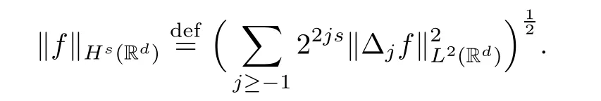
Definition 2.1Lettings∈R,we set

We define the homogeneous Hilbert space

Remark 2.2Lettings∈R,we also set

We can deduce that there exist two positive constantsc0andC0such that

The following Bernstein’s lemma will be repeatedly used throughout this paper:

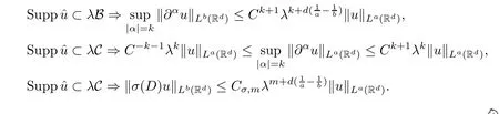
Lemma 2.3Let B be a ball and C a ring of Rd.A constantCexists so that for any positive real numberλ,any non-negative integer k,any smooth homogeneous functionσof degree m,and any couple of real numbers (a,b) with 1 ≤a≤b,it holds that

To prove the main theorem,we need the following lemma concerning the product laws in Sobolev spaces,the proof of which is a standard application based on the Littlewood-Paley theory:

Lemma 2.4(see [1]) Letσ ＞0 andσ1∈R.Then we have,for allu,v∈Hσ(Rd) ∩L∞(Rd),

Lemma 2.5(see [1]) Letσ ＞0 and letfbe a smooth function such thatf(0)=0.Ifu∈Hσ(Rd),then there exists a functionC=C(σ,f,d) such that

Lemma 2.6(see [1]) Letσ ＞and letfbe a smooth function such thatf′(0)=0.Ifu,v∈Hσ(Rd),then there exists a functionC=C(σ,f,d) such that

Lemma 2.7(see [1]) Letσ ＞-1.There exists a positive sequence {cj}j≥-1satisfying‖cj‖?2=1 such that

Lemma 2.8Letσ ＞-1.Suppose thatρ∈Hσ(Rd) andu∈Hσ+1(Rd).Then we have,forj≥0,

where {cj}j≥0satisfies ‖cj‖?2≤1.

ProofIt is easy to get that

On the other hand,it follows,by Lemma 2.4,that

Combining these two inequalities,we have completed Proof of the Lemma 2.8. □

3 A Priori Estimate

In this section,we shall establish the a priori energy estimate for (1.3) which the method is motivated by [34].First,we transform (1.3) into the following linear system:

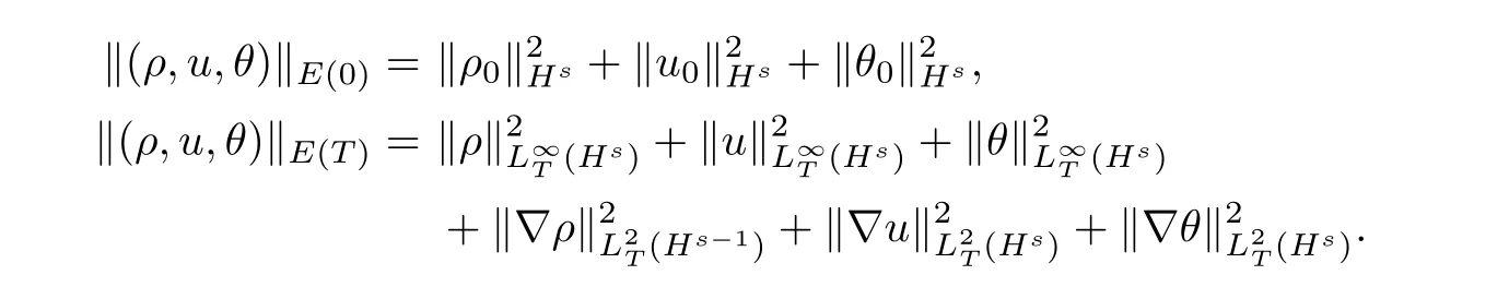
In order to simplify the notation,we define the functional set (ρ,u,θ) ∈E(T) for

The corresponding norms are defined as

Then,we have the following main proposition:

Proposition 3.1Lets ＞,d=2,3 andT ＞0.Let (ρ,u,θ) ∈E(T) be the solution of Cauchy problem (3.1) with initial data (ρ0,u0,θ0).Suppose that ‖ρ(t,·)‖L∞≤and that‖θ(t,·)‖L∞≤Then there exists a positive constant C depending ons,μ(1),κand the smooth functionsμ(x) andκ(x) such that

ProofWe first apply the operator Δjto (3.1) to get

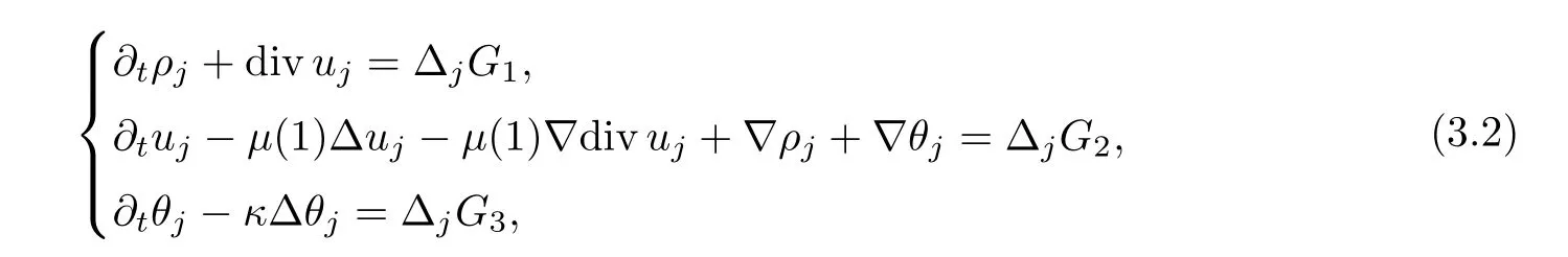
whereρj=Δjρ,uj=Δjuandθj=Δjθ.Letλ ＜be a positive constant to be chosen later.Multiplying the first equation of (3.2) byρj-Δρj-λdivujand integrating by parts,it follows that

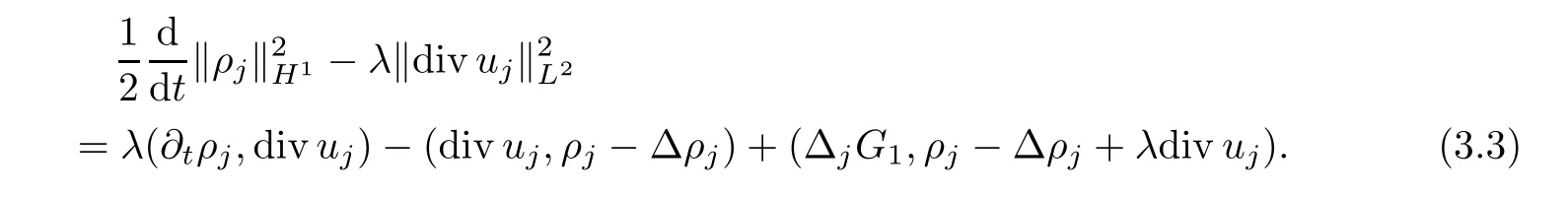
Multiplying the second equation of (3.2) byuj-Δuj+λ?ρjand integrating by parts,we obtain that

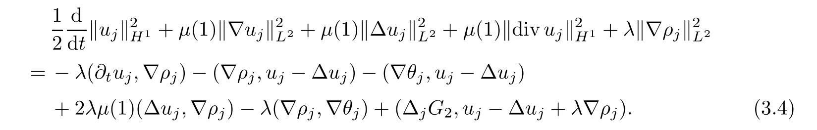
Multiplying the third equation of (3.2) byθj-Δθjand integrating by parts,we have that

we can deduce from (3.3)–(3.5) that

where Λ is a large positive constant to be chosen later.

Note that forj≥0,we have that ‖uj‖L2≤c02-j‖?uj‖L2for somec0＞0.Then,it is not difficult to check,forj≥0,that

Choosingλsmall enough and Λ big enough,and combining (3.7)–(3.9),one can infer from(3.6),for anyj≥0,that

It is not difficult to check,for anyj≥0,it holds that

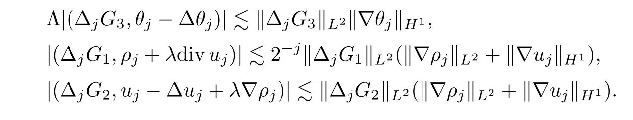
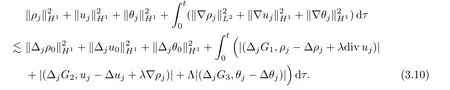
As a result,we can get,by applying Lemma 2.8 and Hlder’s inequality,that

By the same argument as in (3.10),we have that

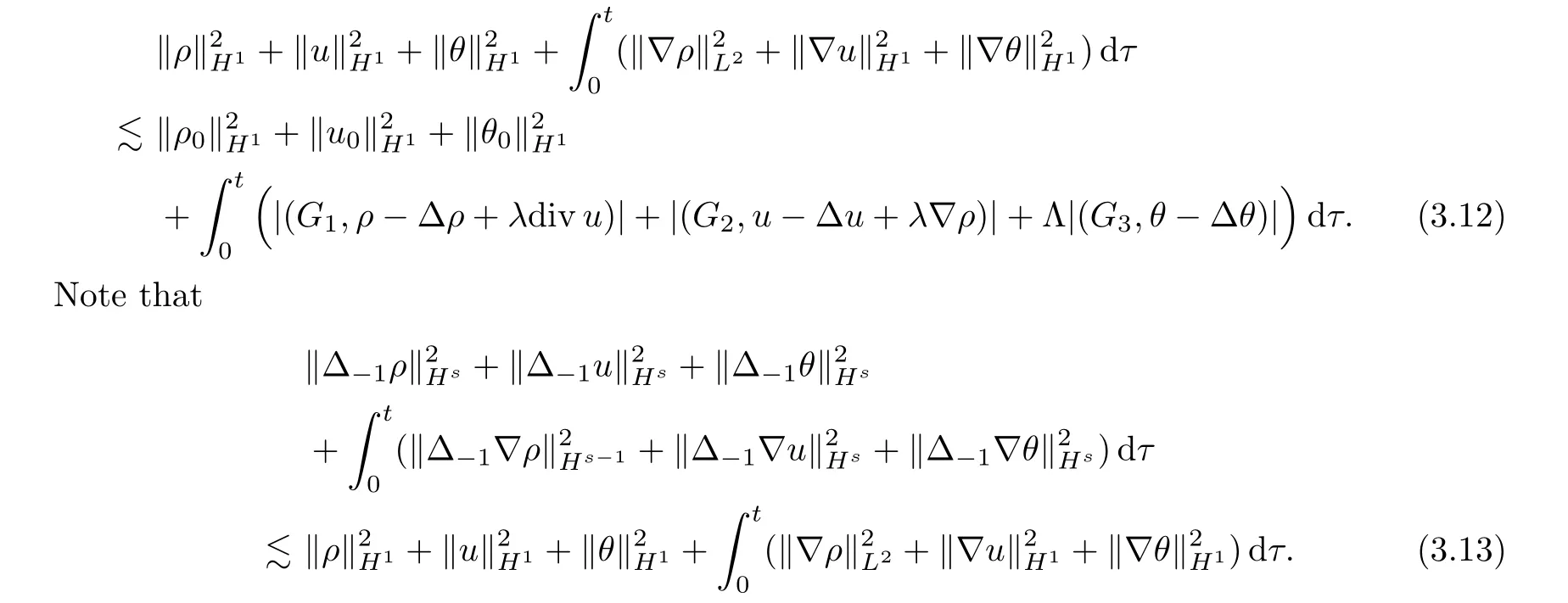
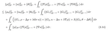
Now,multiplying (3.11) by 22j(s-1)and then summing forj≥0,it follows from (3.12) and(3.13) that

By ‖?u‖L∞?‖?u‖Hswiths ＞and Lemma 2.4,one has

Note that ‖ρ(t,·)‖L∞≤.Then,for any smooth functionf(x) such thatf(0)=0,we have the following inequality:

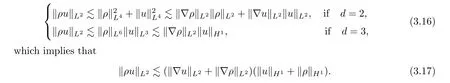
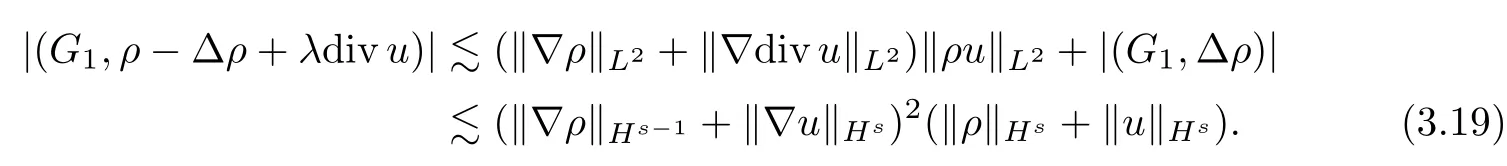
Also,by (3.17),we see that

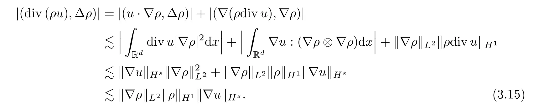
Combining (3.15) and (3.17) implies that

In view of the fact that

Following the same argument as (3.17),we also have that

Applying Lemmas 2.4 and 2.5 once again,and using (3.18) and (3.22),one has

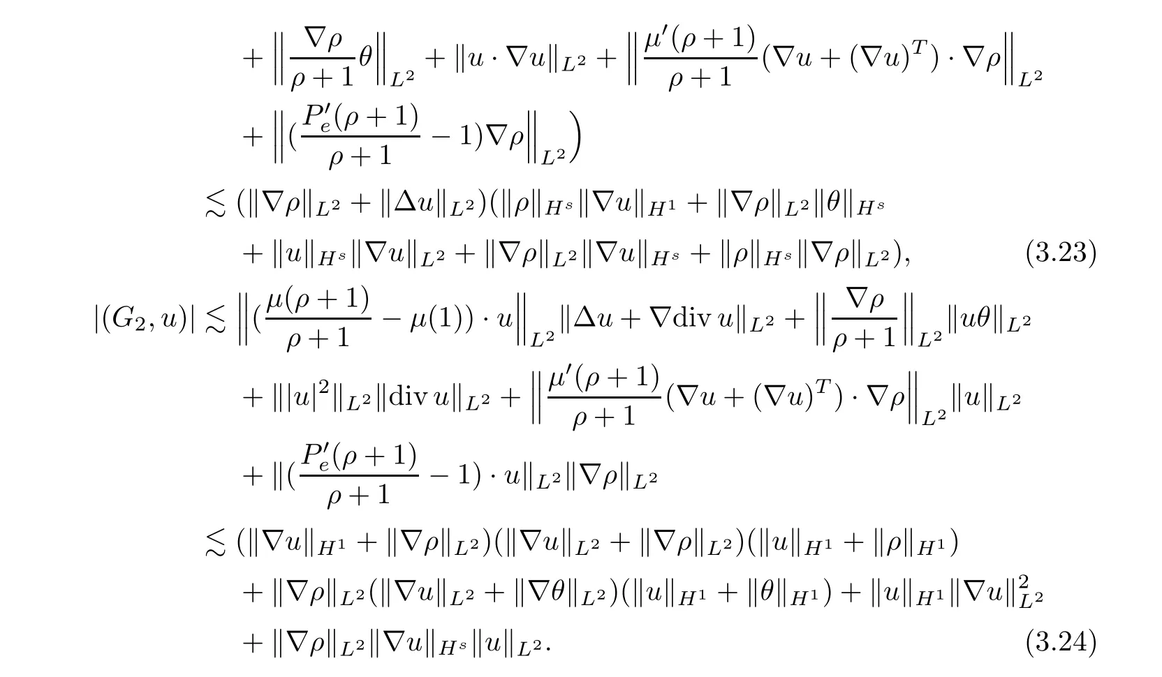
Combining (3.23) and (3.24),we have that

For any 1 ≤q ＜∞,it is easy to see that

which,along with the same argument as in (3.16),leads to

According to Lemma 2.4,and using (3.20) and (3.26),we get

Summing up (3.27) and (3.28),we obtain that

Using Lemma 2.4 gives rise to

By Lemmas 2.4,2.5 and (3.21),we deduce that

Applying Lemma 2.4 and combining (3.20) and (3.21),one has that

Therefore,substituting (3.19),(3.25) and (3.29)–(3.32) into (3.14),and then using Hlder’s inequality,we obtain,for allt∈[0,T],that

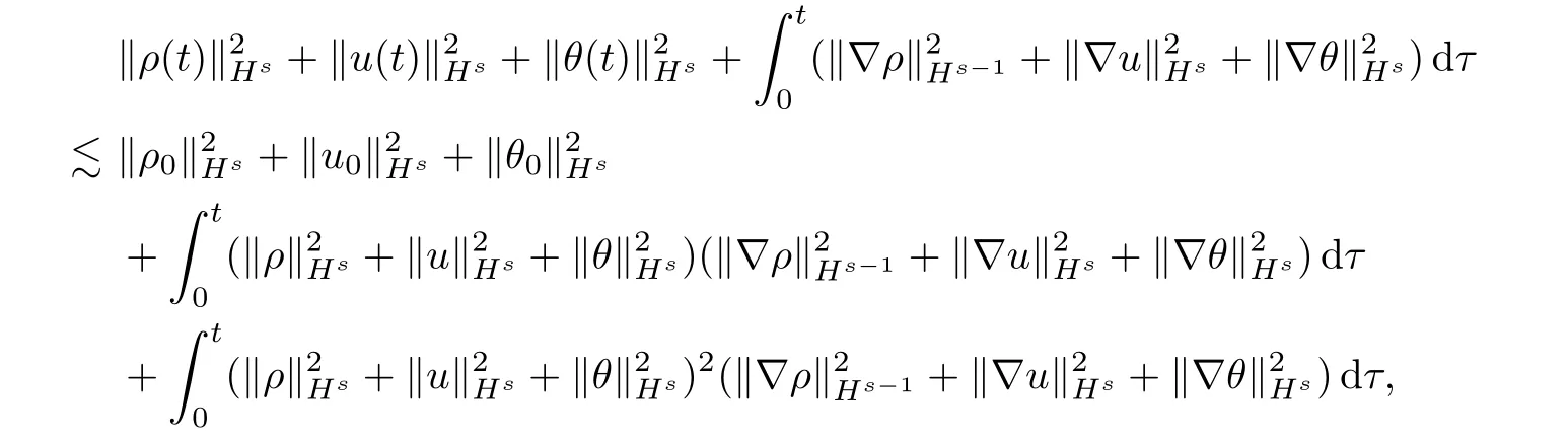
which further implies that

This completes the proof of Proposition 3.1. □

4 Proof of Theorem 1.1

In this section,we shall use four steps to prove the existence and uniqueness of (1.3) with the small initial data.

Step 1 Construction of the approximate solutionsWe first construct the approximate solutions;as in [1],this is based heavily on the classical Friedrich’s method.Defining the smoothing operator

we consider the following approximate system of (1.3) forUε=(ρε,uε,θε):

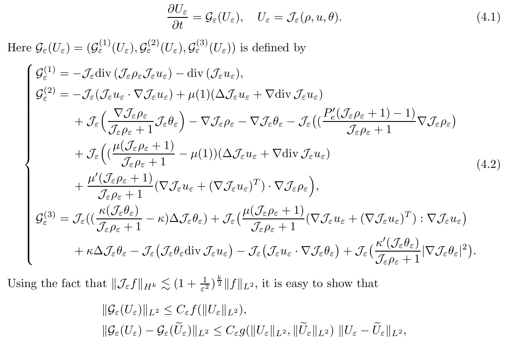
wherefandgare polynomials with positive coefficients.Therefore,the approximate system can be viewed as an ODE system onL2.Then the Cauchy-Lipschitz theorem ensures that there exists a strictly maximal timeTεand a unique solution (ρε,uε,θε) which is continuous in time with a value inL2.,we know that (Jερε,Jεuε,Jεθε) is also a solution of (4.1).Therefore,(ρε,uε,θε)=(Jερε,Jεuε,Jεθε).Thus,(ρε,uε,θε) satisfies the following system:

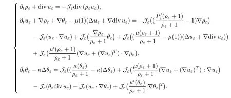
Moreover,we also can conclude that (ρε,uε,θε) ∈E(Tε).

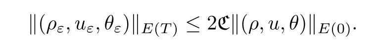
Step 2 Uniform energy estimatesNow,by the losing energy estimate,we will prove that ‖(ρε,uε,θε)‖E(T)is uniformly bounded independently ofε.We assume thatηis small such thatSince the solution depends continuously on the time variable,there exists a positiveT0＜Tεsuch that the solution (ρε,uε,θε) satisfies that

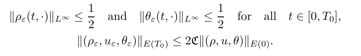
Without loss of generality,we assume thatT0is a maximal time so that the above inequalities hold.In what follows,we will give a refined estimate on [0,T0] for the solution.According to Proposition 3.1,we obtain,for all 0＜T≤T0,that

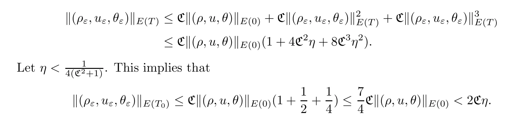
We also assume thatηis small enough such that.A standard bootstrap argument will ensure that,for all 0＜T ＜∞,the following inequality holds:

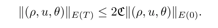
Step 3 Existence of the solutionThe existence of the solution (ρ,u,θ) ∈E(T) of(1.3) can be deduced by a standard compactness argument to the approximation sequence(ρε,uε,θε);we omit it here,for convenience.Moreover,it holds,for all 0＜T ＜∞,that

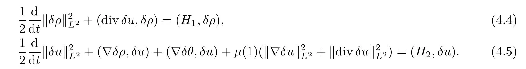
Step 4 Uniqueness of the solutionWe will show that the solution guaranteed by Step 3 is unique.Suppose that (ρ1,u1,θ1) ∈E(T) and (ρ2,u2,θ2) ∈E(T) are two solutions of the system (1.3).Denote thatδρ=ρ1-ρ2,δu=u1-u2andδθ=θ1-θ2.Then,we have that

Multiplying the first equation of (4.3) byδρ,and the second equation of (4.3) byδu,and integrating by parts,we have that

Similarly,multiplying the third equation of (4.3) byδθgives that

In view of (divδu,δρ)+(?δρ,δu)=0,we can deduce from (4.4)–(4.6) that

According to the Sobolev embedding relation,we have,for alla∈H1,b∈Hs-1,that

from which,with Lemmas 2.4 and 2.6,one has that

In what follows,we have to deal with the term (H2,δu) on the right hand side of (4.5).From integration by parts,Hlder’s inequality,and (4.8),the first term in (H2,δu) can be bounded as

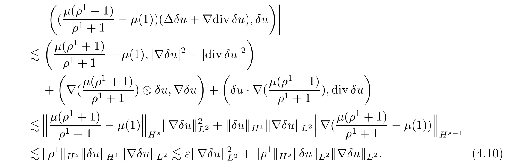
In a similar manner,we can get that

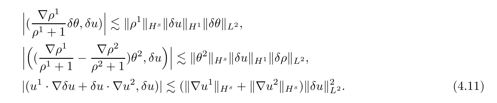
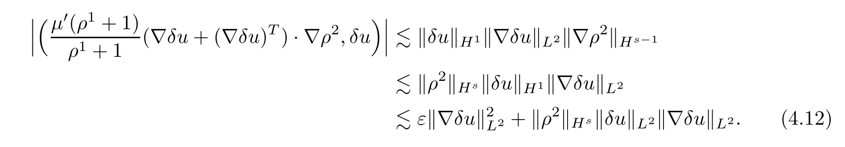
The rest of the terms in (H2,δu) can be dealt in a manner similar to that above,so here we omit the details.We now have that

where V(t) depends on ‖ρ1‖Hs,‖ρ2‖Hs,‖u1‖Hs+1,‖u2‖Hs+1,‖θ1‖Hs+1,‖θ2‖Hs+1.

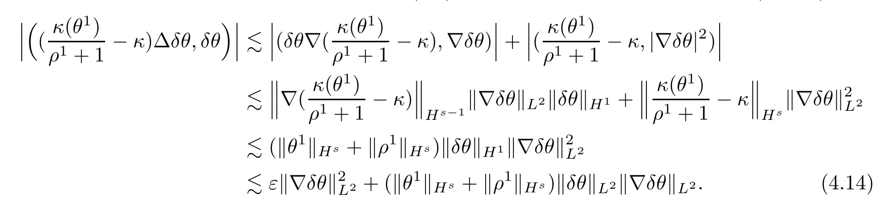
Now,we begin to estimate the terms in (H3,δθ) one by one.Using integration by parts,Hlder’s inequality,Young’s inequality and (4.8),we can bound the first term in (H3,δθ) as

The second term in (H3,δθ) can be bounded directly from Hlder’s inequality and (4.8) such that

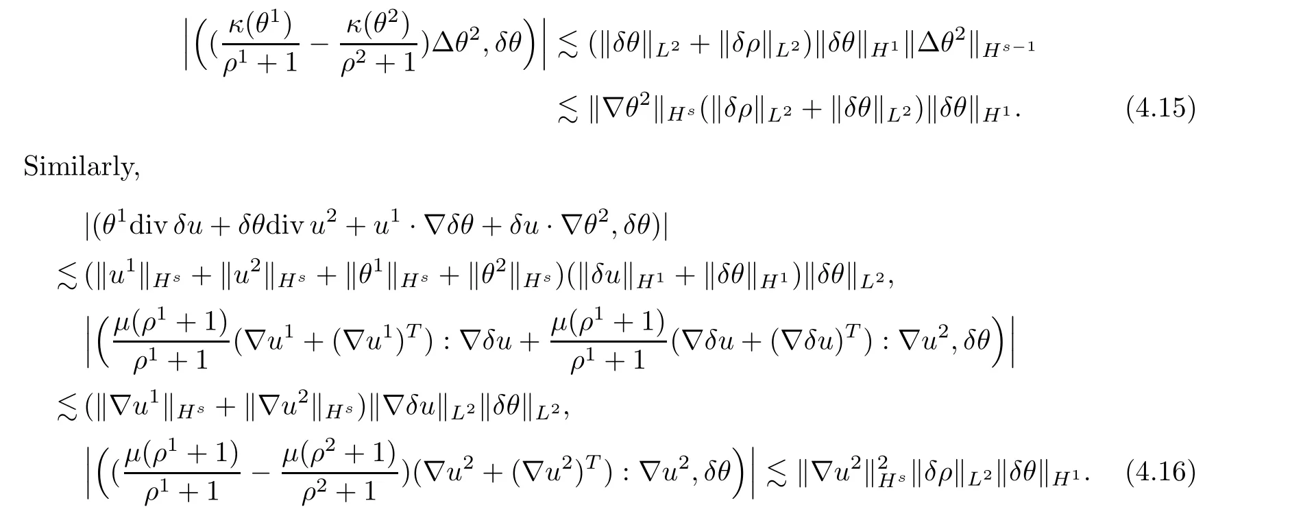
The last two terms in (H3,δθ) can be estimated from Lemmas 2.4 and 2.6,(3.21) and (4.8)such that

Combining the inequalities (4.14)–(4.17),we have that

where W(t) depends on ‖ρ1‖Hs,‖ρ2‖Hs,‖u1‖Hs+1,‖u2‖Hs+1,‖θ1‖Hs+1,‖θ2‖Hs+1.

Therefore,inserting (4.9),(4.13) and (4.18) into (4.7),we finally deduce that

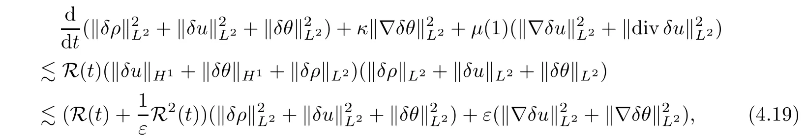
where R(t) depends on ‖ρ1‖Hs,‖ρ2‖Hs,‖u1‖Hs+1,‖u2‖Hs+1,‖θ1‖Hs+1,‖θ2‖Hs+1.Now,choosingεsmall enough,and according to Gronwall’s inequality,(4.19) implies that (δρ(t),δu(t),δθ(t))=(0,0,0) for allt∈[0,∞).This completes the proof of the uniqueness of the solution to system (1.3).