Two regularization methods for identifying the source term problem on the time-fractional diffusion equation with a hyper-Bessel operator
2022-08-25 08:52:54FanYANG楊帆QiaoxiSUN孫喬夕XiaoxiaoLI李曉曉
Fan YANG(楊帆)+Qiaoxi SUN(孫喬夕)Xiaoxiao LI (李曉曉)
Department of Mathematics,Lanzhou University of Technology,Lanzhou 730000,China E-mail: gufggd114@163.com; qiaoxisunlaut@163.com; liaiaoriaogood@126.com.
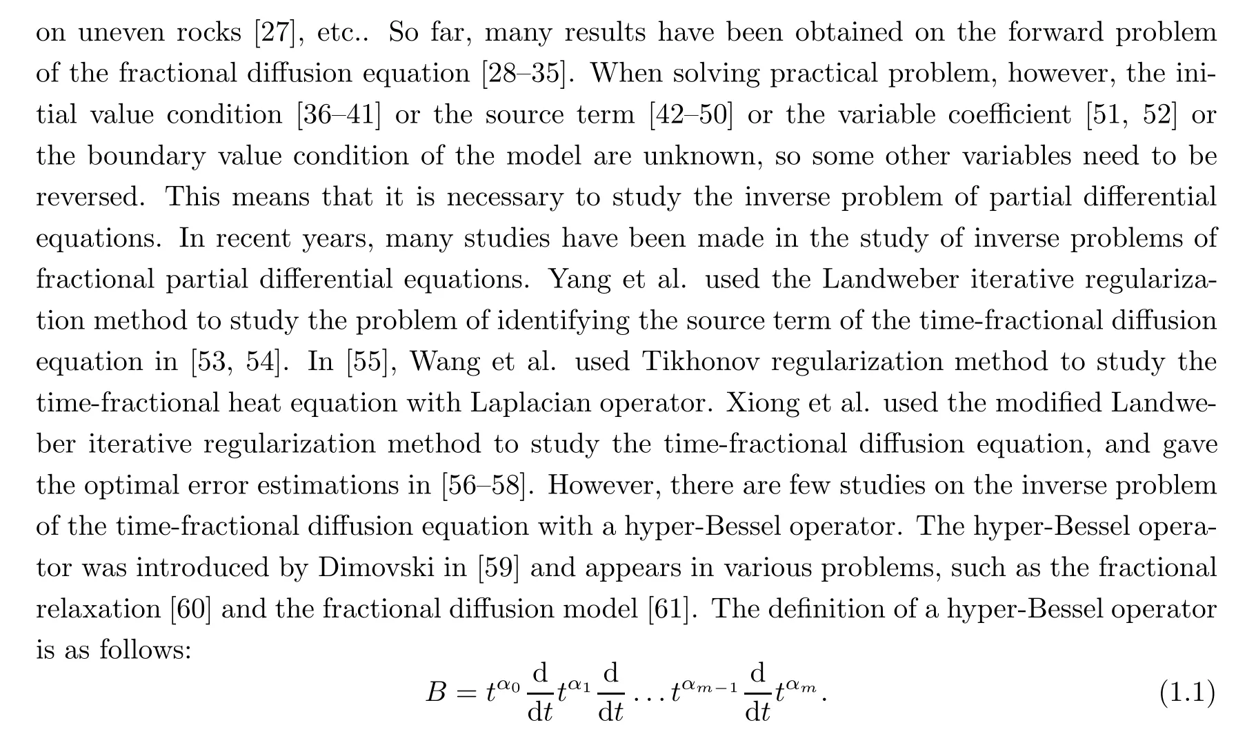
Nguyen Huy Tuan et al. [62]considered the initial value problem of the time-fractional diffusion equation with hyper-Bessel operator, gave the existence and regularity of the solution for the inverse problem, and obtained the corresponding H¨older-type error estimation under different regularization parameter selection rules. In [63], they considered the inverse problem of identifying the source term of the time-fractional diffusion equation, in which the time-fractional operator is replaced by a regular hyper-Bessel operator, and gave the existence of the source term and the conditional stability. The error estimates under the selection of a priori and a posterior regularization parameters were given, but the error estimations were saturated, and the order of error estimations was not optimal.
In this article, we give the optimal error analysis of this inverse problem, and present the error estimates under the fractional Tikhonov regularization method and the fractional Landweber iterative regularization method. Combining this with the optimal order theorem,we find that the error estimate obtained by the fractional Tikhonov regularization method is saturated,and the error estimates are not of the order optimal for all p,while the error estimate under the fractional Landweber regularization method obtained is not saturated and the order is optimal for all p. In this paper, we consider the following time-fractional diffusion equation with a hyper-Bessel operator:
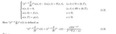
where 0 <α <1, 0 <β <1, Γ(x) is a Gamma function, and T >0 is a fixed value. When β = 1, this operator coincides with the R-L fractional derivation. If F(x,t) is known, the problem(1.2) is a forward problem. If F(x,t) is unknown, problem(1.2) is an inverse problem.In this paper, we identify the unknown source term by using the final value data of t = T.Assume that we have the source term F(x,t)=F(x)Q(t), where Q(t)is known in advance. We then want to identify the unknown source term F(x) by using the value of the final time T.In fact, the observation data g(x) is obtained by measurement, and the measurement data is noised. The exact data g(x) and the measurement data gδ(x) satisfy

The rest of this article is organized as follows: in Section 2, some auxiliary propositions are introduced. In Section 3, we give the ill-posedness and conditional stability of the inverse problem. In Section 4, the optimal error bound for the inverse problem is given. Section 5 and Section 6 give the error estimates under the a priori and a posteriori regularization parameter selection rules of the fractional Tikhonov regularization method and the fractional Landweber iterative regularization method. In the last section,numerical examples are given to prove that the two regularization methods are effective for restoring the stability of the inverse problem.
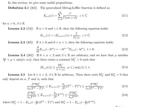
2 Auxiliary Propositions
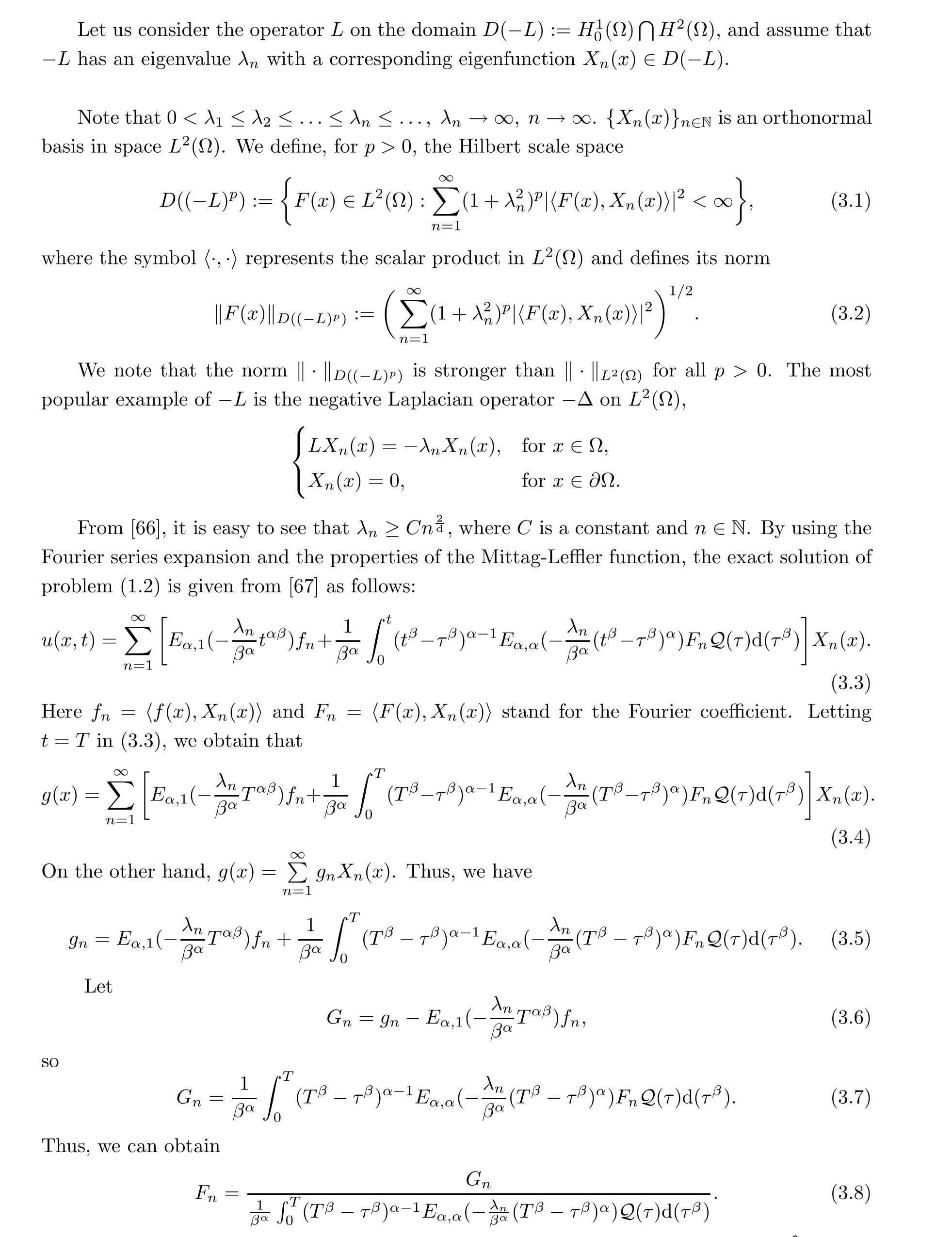
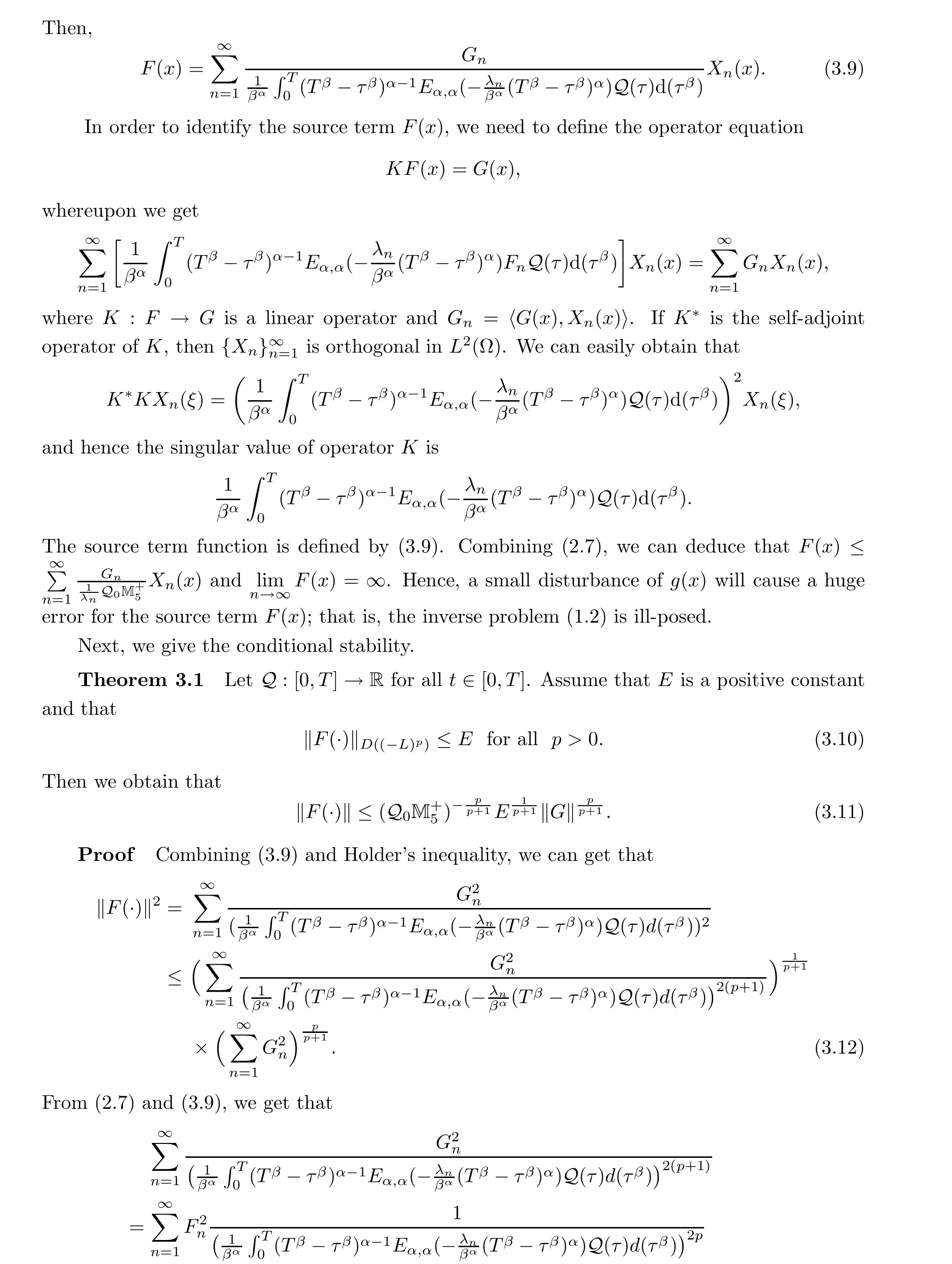
3 Ill-Posedness of the Problem and the Conditional Stability of (1.2)
4 Preliminary Results and Optimal Error Bounds for Problem (1.2)
4.1 Preliminary results
Let X and Y be two Hilbert spaces. Problem(1.2)can be transferred to solve the following operator equation:
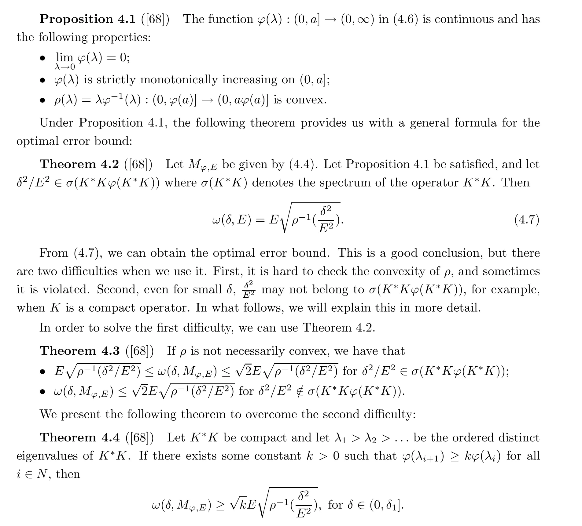
If Theorems 4.2 and 4.3 are satisfied,we can obtain an optimal error bound for the problem(1.2).
4.2 Optimal error bound for problem (1.2)
In this subsection, we will give the optimal error bound for the inverse problem (1.2). We only focus on recovering F(x) from noisy data gδ∈L2(Ω) provided that
Remark 4.9 In general,the source condition(3.4)is difficult to verify for practical problems since the index function φ cannot be known explicitly. However,in our consideration,the a priori source condition u(x,0)∈Mφ,Eis equivalent to u(x,0)∈Mp,E, and it is easy to verify the latter since the unknown function u(x,0) has p order smoothness.
Remark 4.10 The index function φ(see p.4 in[33])can be derived in three stages. First,to obtain the convergence estimate, we need some smoothness assumption for the solution(e.g.(3.18)). The smoothness assumption is often given in the form of a familiar Sobolev norm,for example, in the Hpnorm. Second, we can formulate the inverse problem as an operator equation. Using the singular values (which exist in most cases) of the obtained operator, we can rewrite the smoothness assumption in the variable Hilbert scale (similar to (3.23), or see p. 791 in [38]). Third, comparing the smoothness assumption in a variable Hilbert scale and the source condition (3.4), we can easily get the implicit expression of the index function. For details, we refer the reader to [33]. For the self-adjoint compact operator in particular, the above procedure may be simpler; see the examples in [33].
5 The Fractional Tikhonov Regular Method and the Convergence Error Estimate
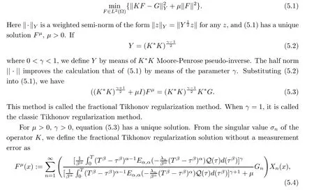
Huo proposed the following regularization method in[70],its essence being the least squares problem with penalty:
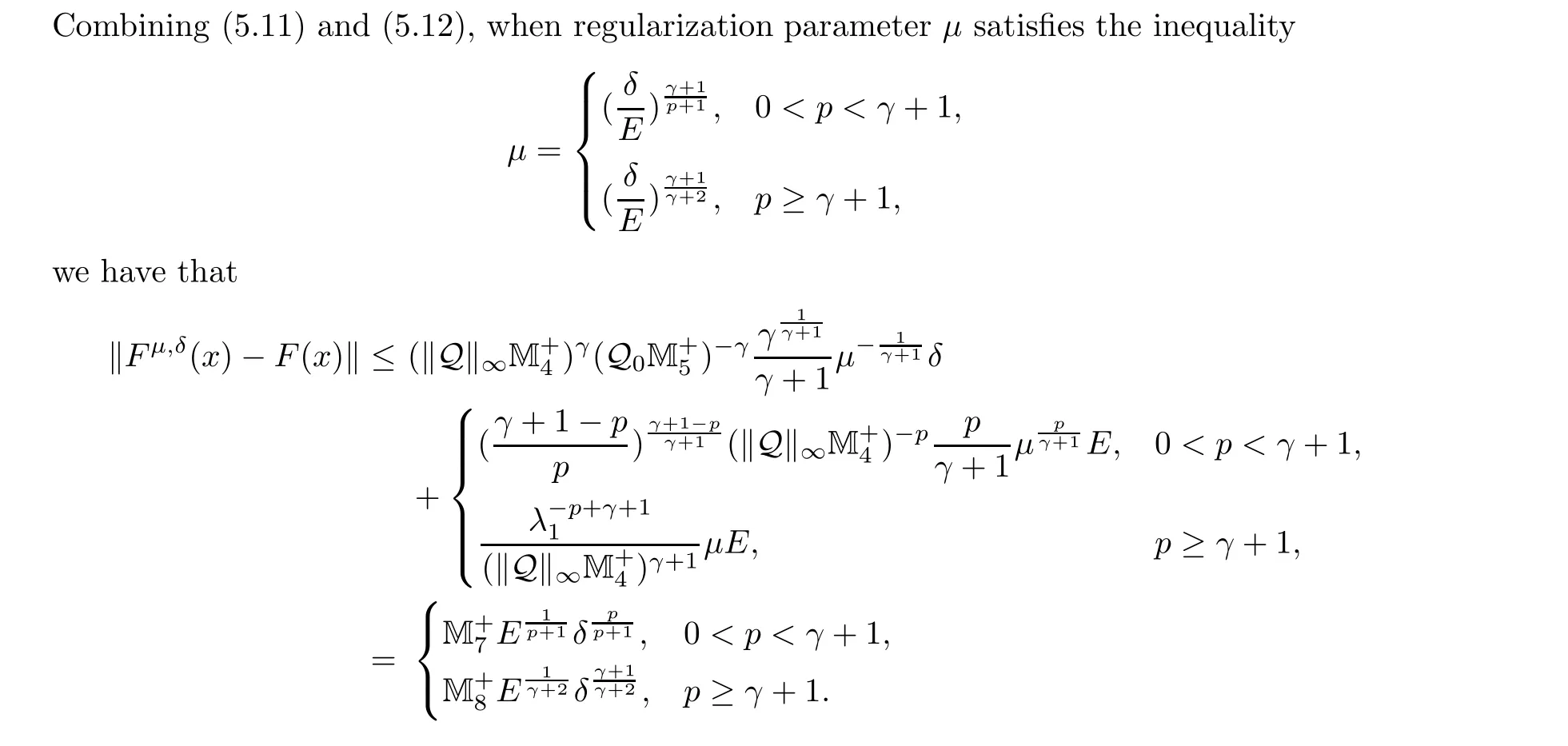
5.1 Error estimate under an a priori parameter choice rule
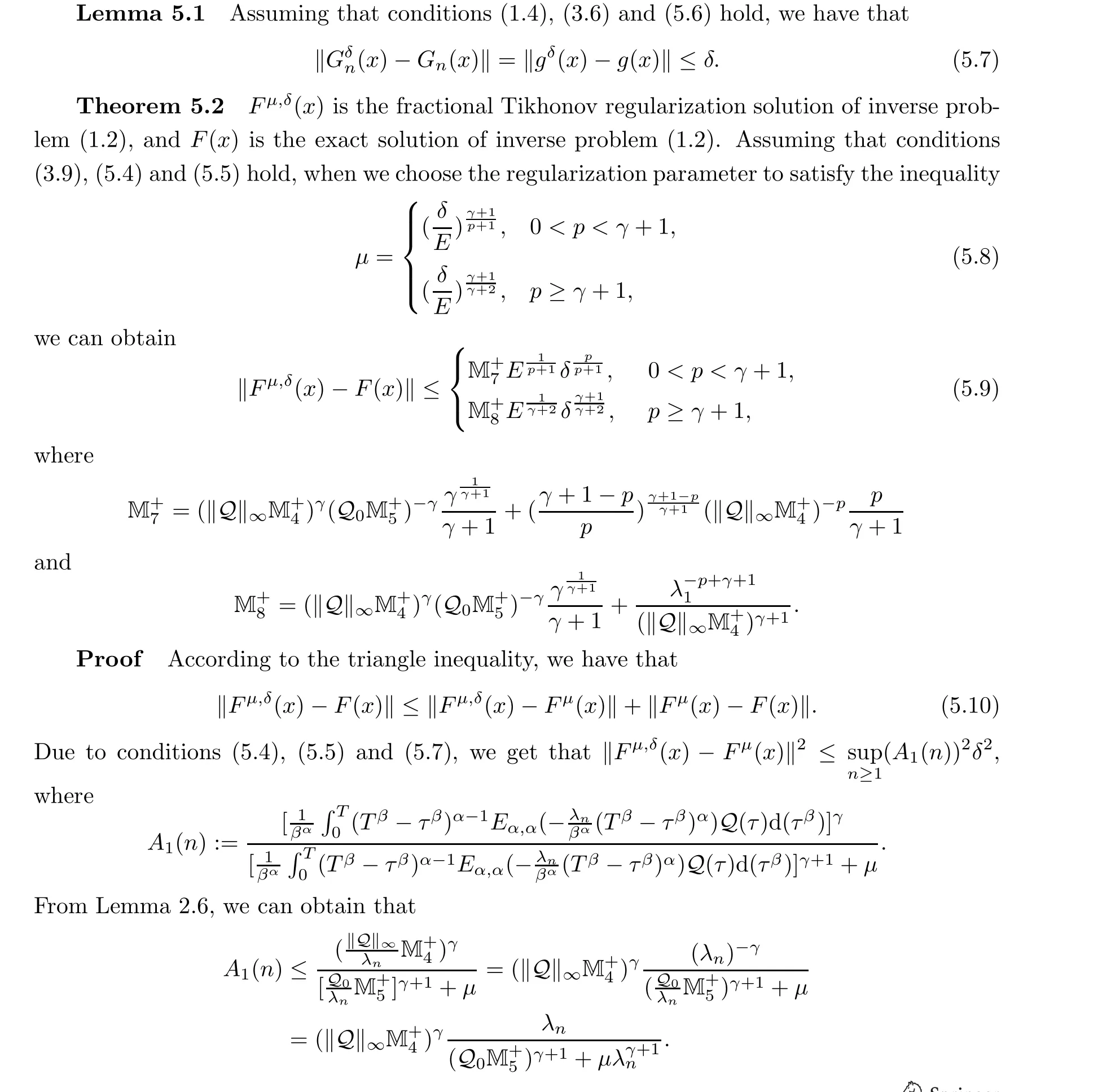
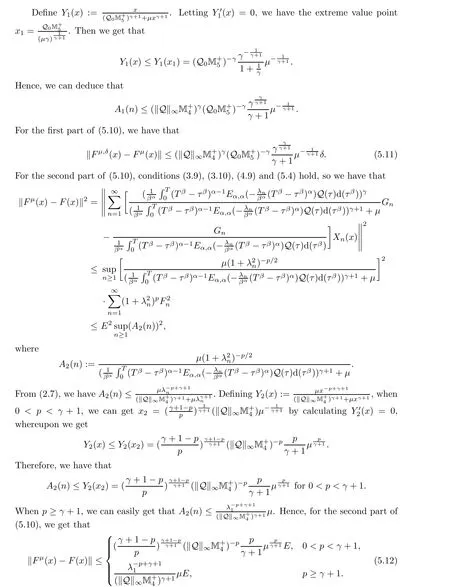
The proof is completed. □
Remark 5.3 Combining Theorems 4.8 and 5.2,we know that the error estimate obtained by the fractional Tikhonov regularization method under the a priori regularization parameter selection rule is of the optimal order for 0 <p <γ+1.
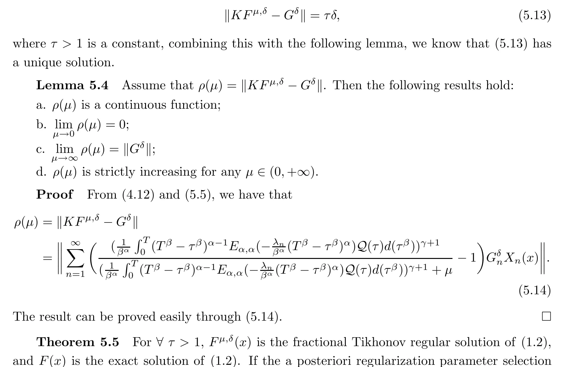
5.2 A posteriori parameter choice rule and convergent estimate
In this subsection, we choose a posteriori regularization parameter μ by using Morozov’s discrepancy principal. We have that μ satisfies
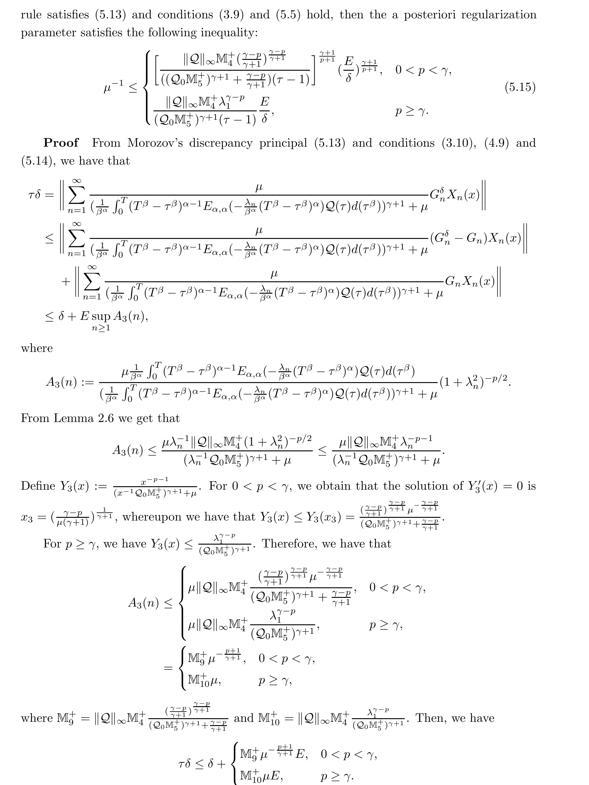
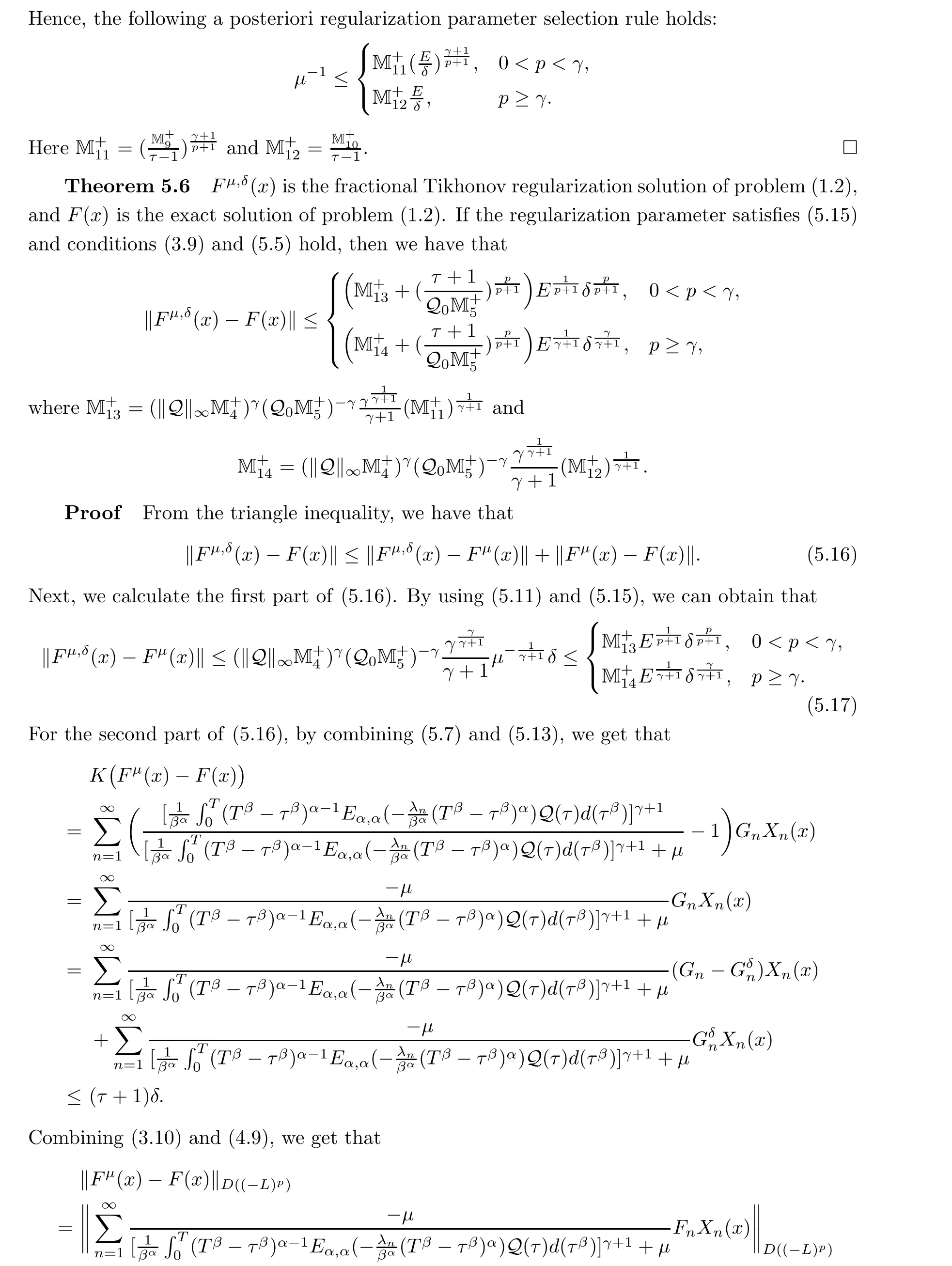
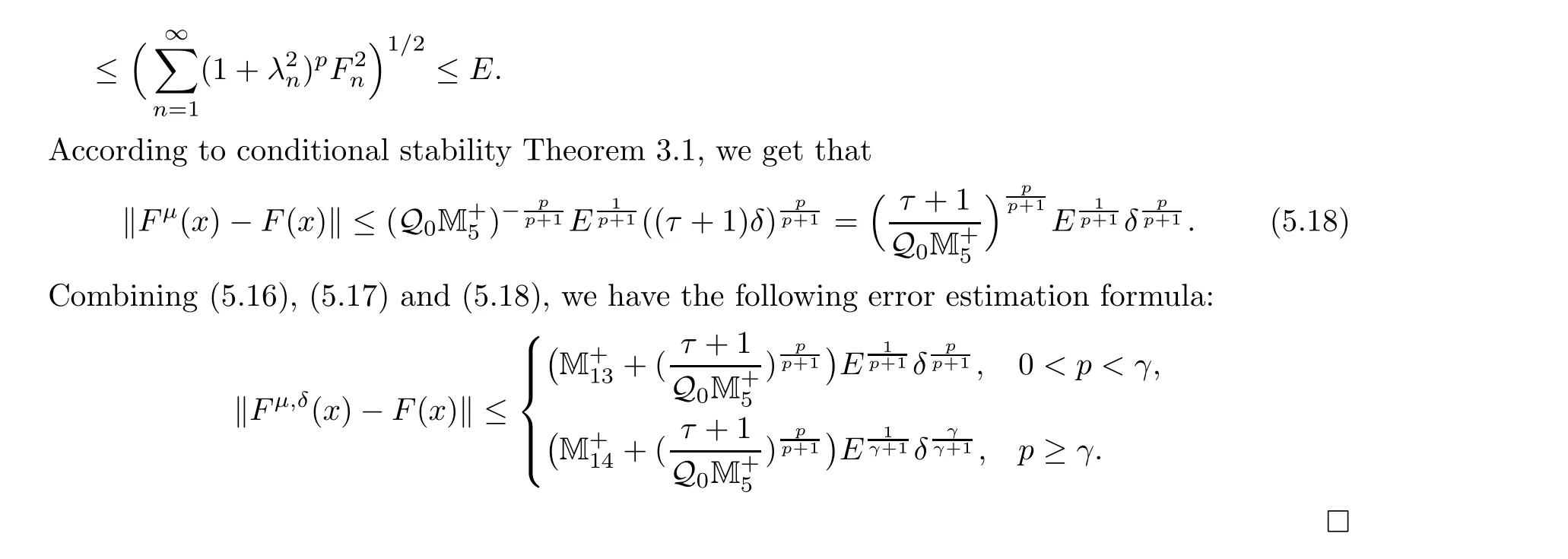
Remark 5.7 Combining Theorems 4.8 and 5.3, we know that the error estimate obtained by the fractional Tikhonov regularization method under the a posteriori regularization parameter selection rule is of the optimal order for 0 <p <γ.
Remark 5.8 The error estimate obtained by the fractional Tikhonov regularization method is saturated. When p is a certain value and 0 <γ <1, the order of the measurement error δ in the error estimation formula is certain, as opposed to when p is increasing or decreasing.Therefore, in the next chapter, we propose a fractional Landweber regularization method in order to improve the deficiencies of the above method.
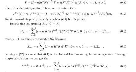
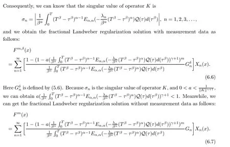
6 The Fractional Landweber Regularization Method and the Convergent Error Estimate
In this section, we use the fractional Landweber regularization method to obtain the regularization solution of the inverse problem (1.4), and KF = G is replaced by the operator equation
6.1 Error estimate under an a priori parameter choice rule
Remark 6.2 Combining Theorems 4.8 and 6.1,we know that the error estimate obtained by the fractional Landweber iterative regularization method under the a priori regularization parameter selection rule is of the optimal order for all p >0.
6.2 The a posteriori parameter choice rule and the convergent estimate
In this subsection,we choose a posteriori parameter m by using the Morozov Principle,and the a posteriori parameter choice rule satisfies that
The proof of the theorem is completed. □
Remark 6.6 Combining Theorems 4.8 and 6.5,we know that the error estimate obtained by the fractional Landweber iterative regularization method under the a posteriori regularization parameter selection rule is of the optimal order for all p >0.
7 Numerical Implementation and Numerical Examples
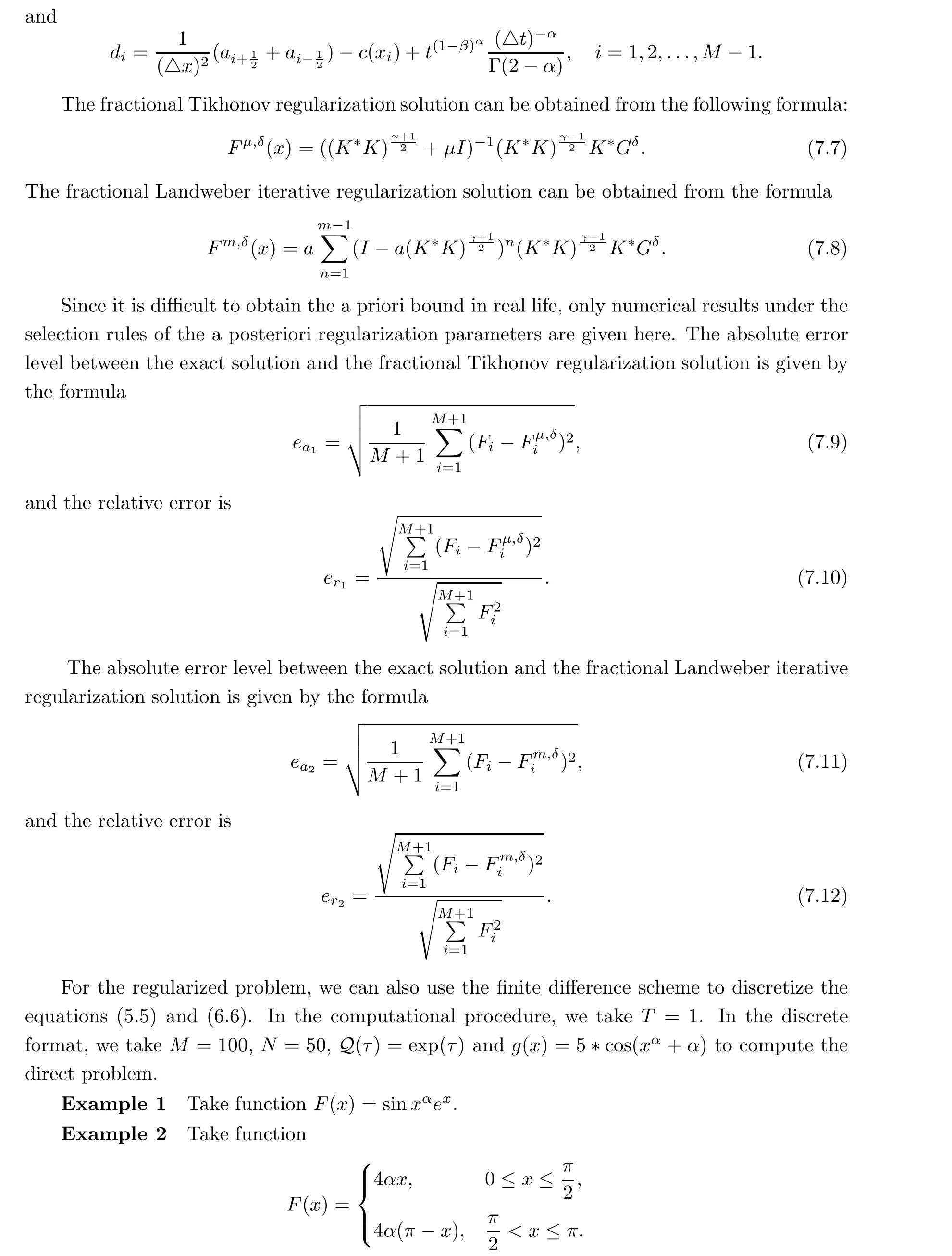
In this section, several numerical examples are given to illustrate the effectiveness of the fractional Tikhonov regularization method and the fractional Landweber iterative regularization method. First,we can obtain g(x)from the initial value f(x)by solving the direct problem as follows:

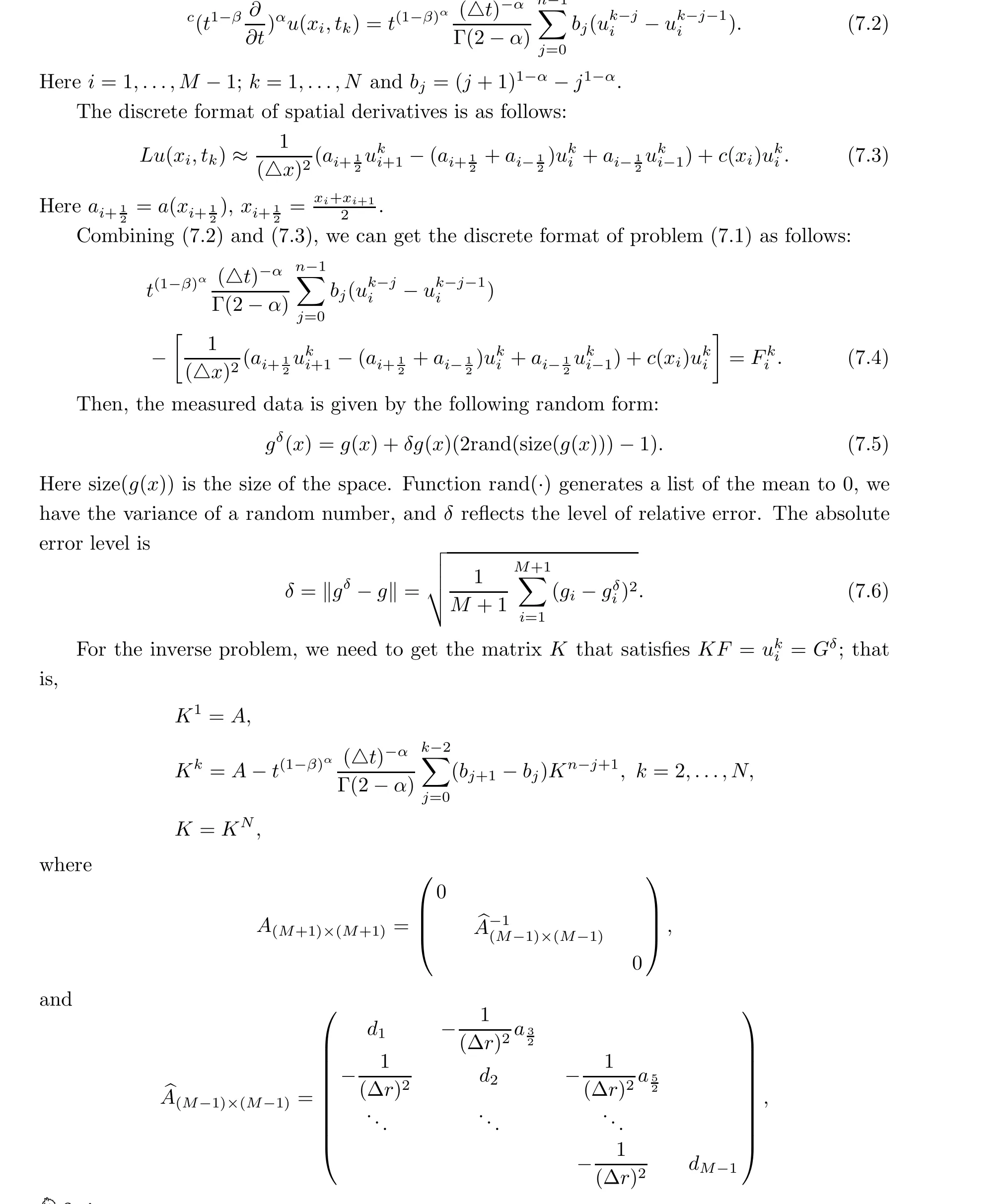
We use the finite difference method to discretize problem(7.1). We assume that Ω=(0,π).Let Δt=T/N and Δx=π/M be the step sizes for time and space variables,respectively. The grid points in the time interval are labelled tk= kΔt, k = 0,1,...,N, the grid points in the space interval are xi=iΔx, i=0,1,...,M, and we set uki=u(xi,tk).
The discrete format of time fractional derivatives is as follows:
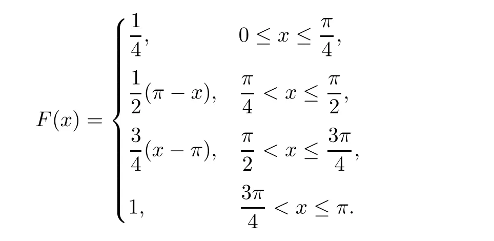
Example 3 Take function
In Figure 1, we give the numerical results of Example 1 under the a posteriori parameter choice rule for various noise levels δ = 0.001,0.0001,0.00001 in the case where α =0.05,0.15,0.25. It can be seen that the numerical error also decreases when the noise is reduced; the smaller α, the better the approximate effect.
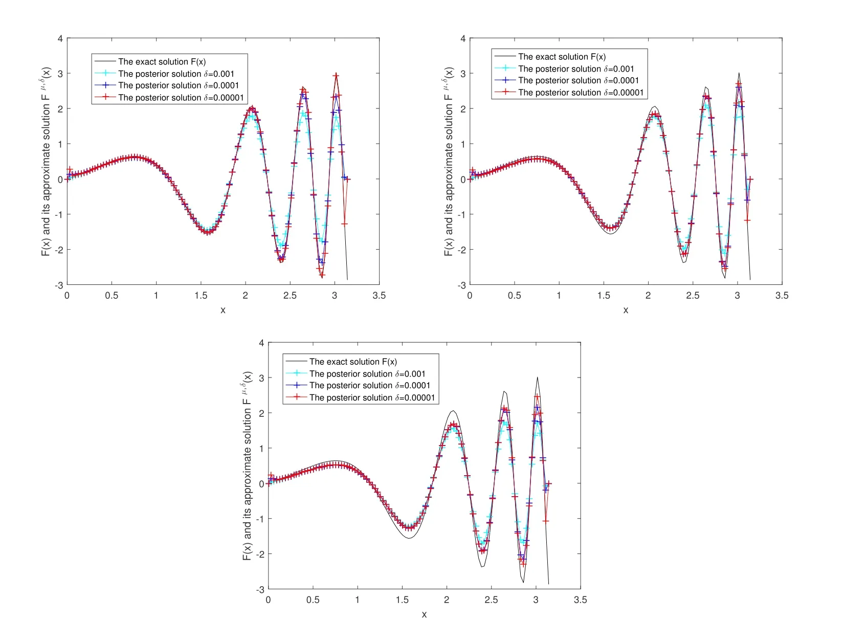
Figure 1 The exact solution and fractional Tikhonov regularization solution Fμ,δ(x) by using the a posteriori parameter choice rule for Example 1: (a) α = 0.05, (b)α=0.15, (c) α=0.25
In Figure 2, we give the numerical results of Example 1 under the a posteriori parameter choice rule for various noise levels δ = 0.01,0.008,0.005 in the case of α = 0.2,0.5,0.8. It can be seen that the numerical error also decreases when the noise is reduced; the smaller α, the better the approximate effect.
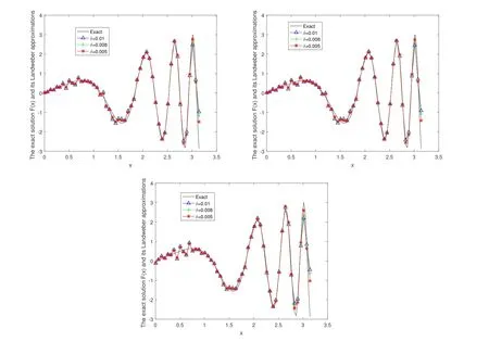
Figure 2 The exact solution and fractional Landweber iterative regularization solution Fm,δ(x)by using the a posteriori parameter choice rule for Example 1: (a)α=0.2,(b) α=0.5, (c) α=0.8
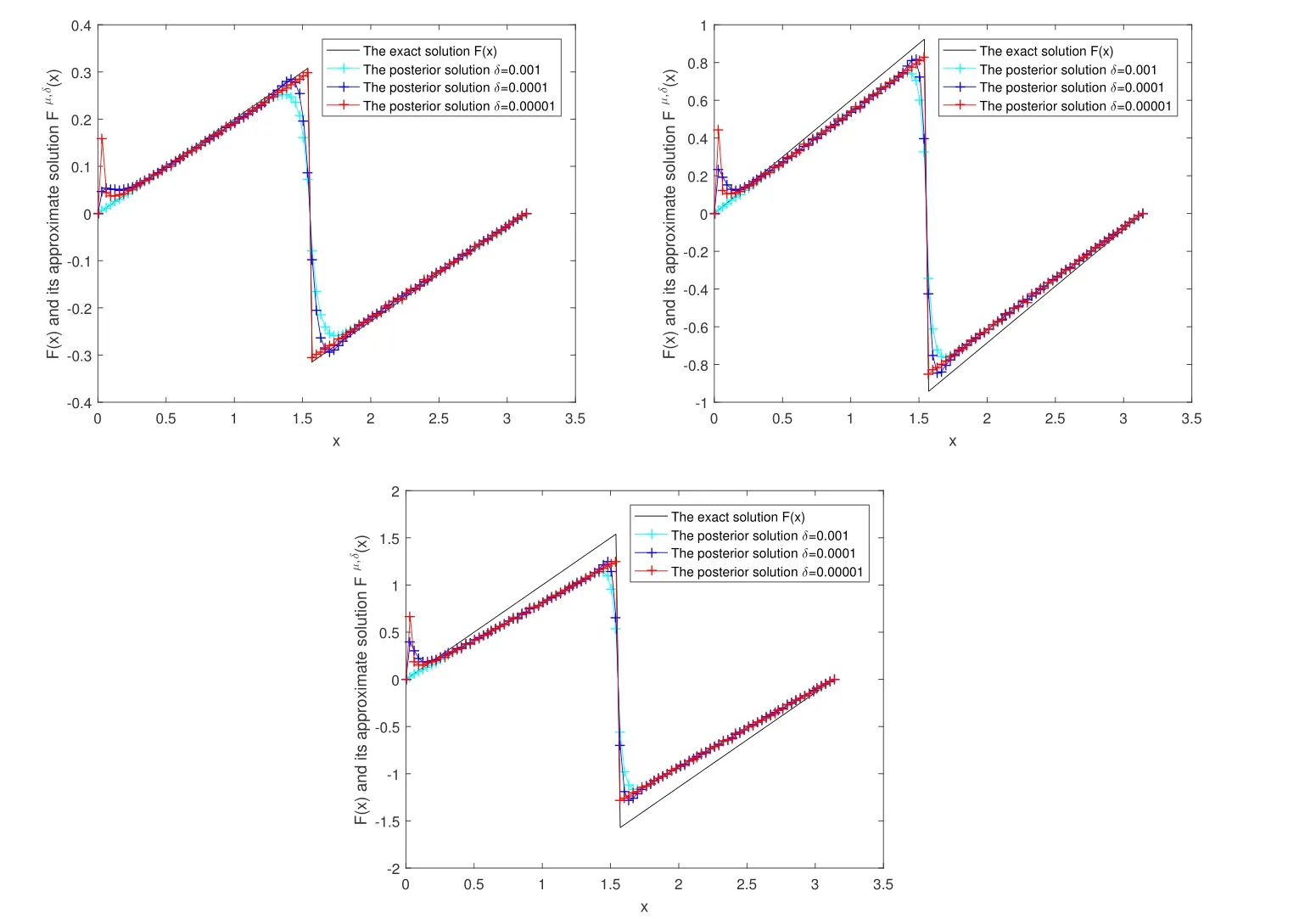
Figure 3 The exact solution and the fractional Tikhonov regularization solution Fμ,δ(x) by using the a posteriori parameter choice rule for Example 2: (a) α = 0.05, (b)α=0.15, (c) α=0.25
In Figure 3, we give the numerical results of Example 2 under the a posteriori parameter choice rule for various noise levels δ =0.001,0.0001,0.00001 in the case of α=0.05,0.15,0.25.It can be seen that the numerical error also decreases when the noise is reduced; the smaller α,the better the approximate effect.
In Figure 4, we give the numerical results of Example 2 under the a posteriori parameter choice rule for various noise levels δ = 0.01,0.008,0.005 in the case of α = 0.2,0.5,0.8. It can be seen that the numerical error also decreases when the noise is reduced; the smaller α, the better the approximate effect.
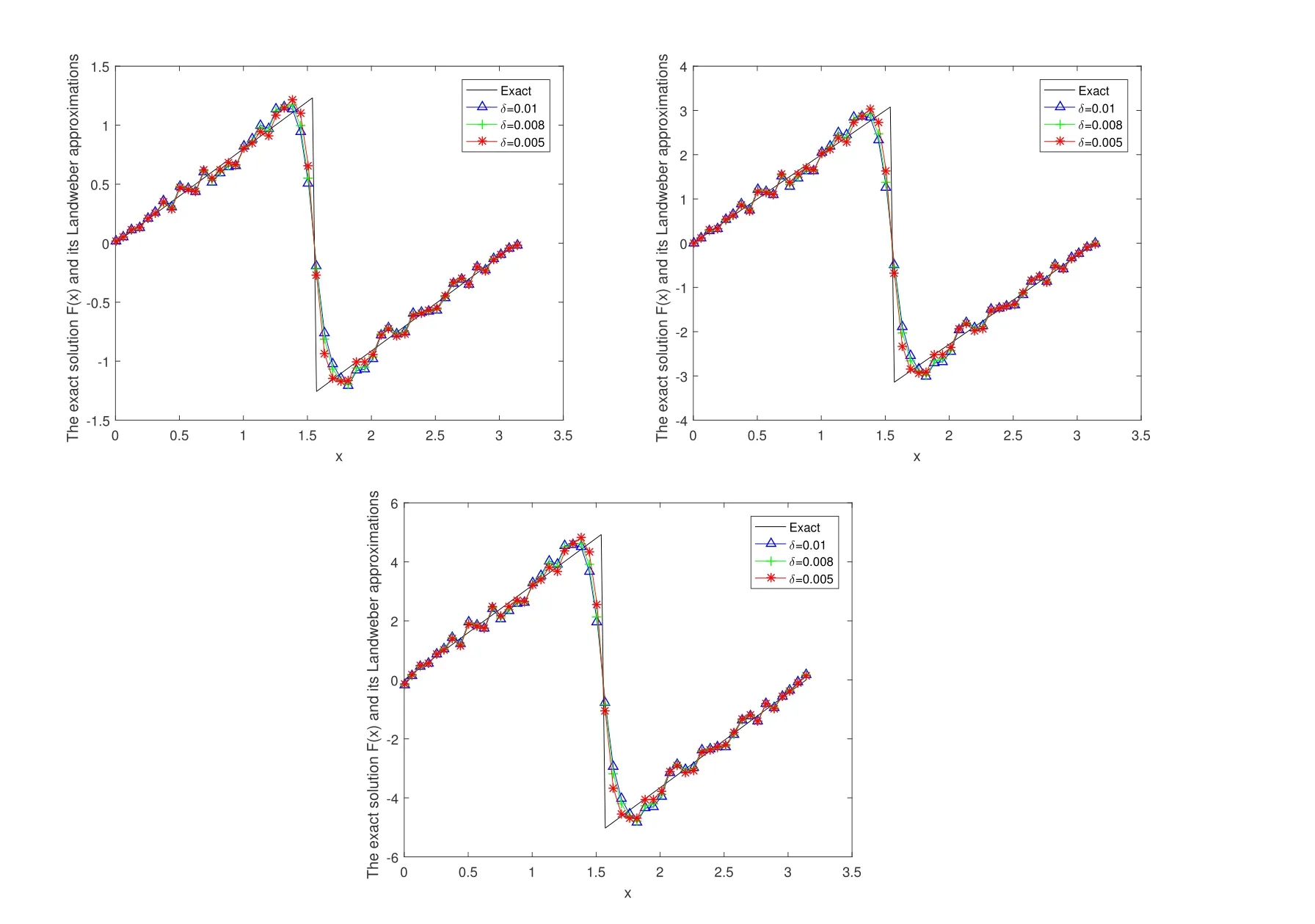
Figure 4 The exact solution and the fractional Landweber iterative regularization solution Fm,δ(x)by using the a posteriori parameter choice rule for Example 2: (a)α=0.2,(b) α=0.5, (c) α=0.8
In Figure 5, we give the numerical results of Example 3 under the a posteriori parameter choice rule for various noise levels δ =0.001,0.0001,0.00001 in the case of α=0.05,0.15,0.25.It can be seen that the numerical error also decreases when the noise is reduced; the smaller α,the better the approximate effect.
In Figure 6, we give the numerical results of Example 3 under the a posteriori parameter choice rule for various noise levels δ = 0.01,0.008,0.005 in the case of α = 0.2,0.5,0.8. It can be seen that the numerical error also decreases when the noise is reduced; the smaller α, the better the approximate effect.
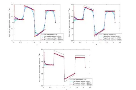
Figure 5 The exact solution and fractional Tikhonov regularization solution Fμ,δ(x) by using the a posteriori parameter choice rule for Example 3: (a) α = 0.05, (b)α=0.15, (c) α=0.25
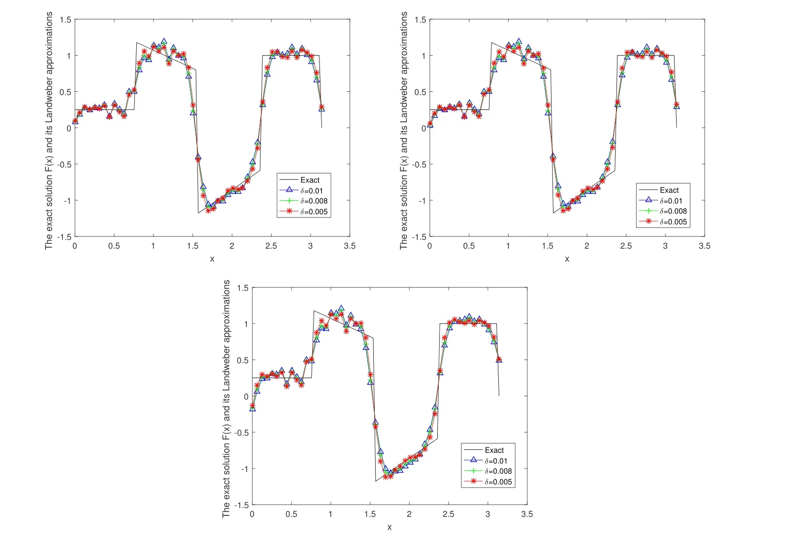
Figure 6 The exact solution and fractional Landweber iterative regularization solution Fm,δ(x)by using the a posteriori parameter choice rule for Example 3: (a)α=0.2,(b) α=0.5, (c) α=0.8
Table 1, Table 2 and Table 3 show the number of iterative steps under the Landweber and the fractional Landweber iterative regularization methods for Example 1, Example 2 and Example 3,respectively. We find that the fractional Landweber iterative regularization method has fewer iteration steps than the Landweber iterative regularization method. From Table 4,Table 5 and Table 6, we find that the smaller the α, the smaller the error behaviour, and the better the numerical simulation for the fixed δ, and the smaller the δ, the smaller the error behaviour, and the better the numerical simulation for the fixed α. When α and δ are fixed, the fractional Landweber iterative regularization method has less error behaviour than the fractional Tikhonov regularization method, so we can infer that the fractional Landweber iterative regularization method is more effective than the fractional Tikhonov regularization method for restoring stability and identifying the source term problem.
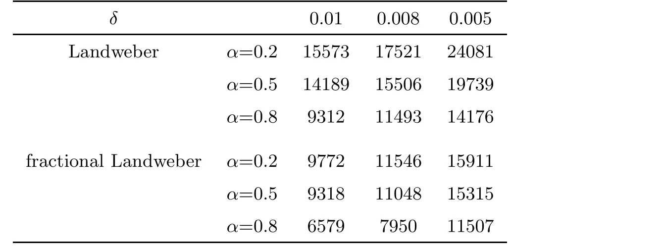
Table 1 The iteration steps of Example 1 for the Landweber iterative and the fractional Landweber iterative regularization methods
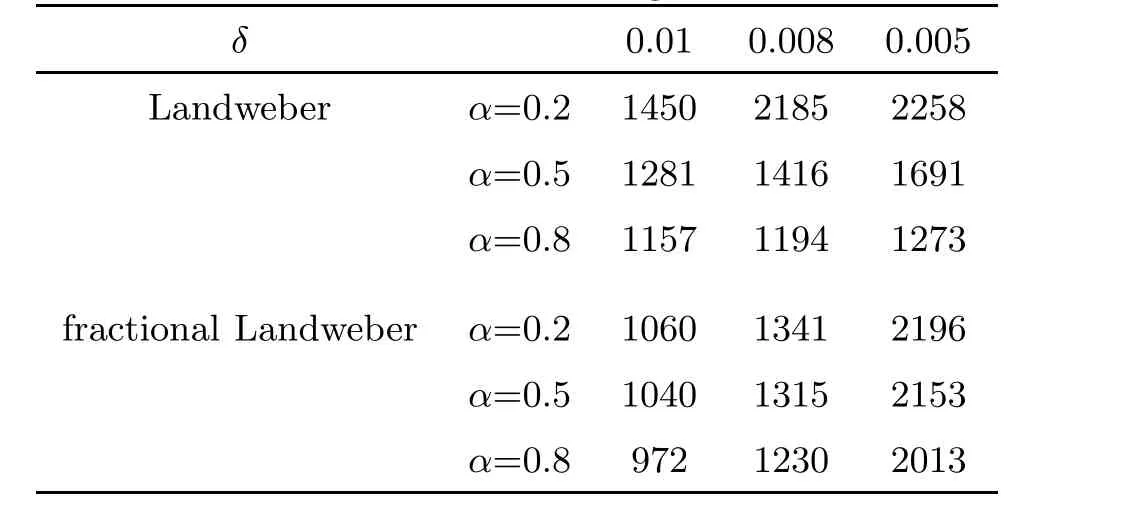
Table 2 The iteration steps of Example 2 for the Landweber iterative and the fractional Landweber iterative regularization methods
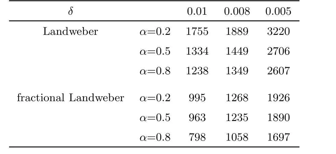
Table 3 The iteration steps of Example 3 for the Landweber iterative and the fractional Landweber iterative regularization methods
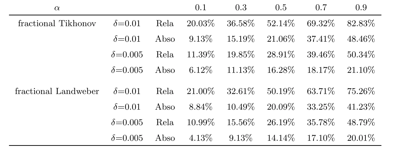
Table 4 Error behaviour of Example 1 for different α with δ =0.01,0.005
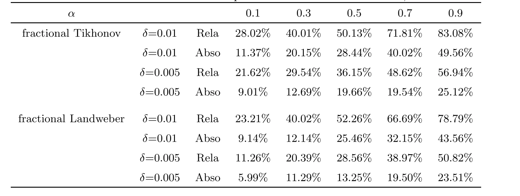
Table 5 Error behaviour of Example 2 for different α with δ =0.01,0.005
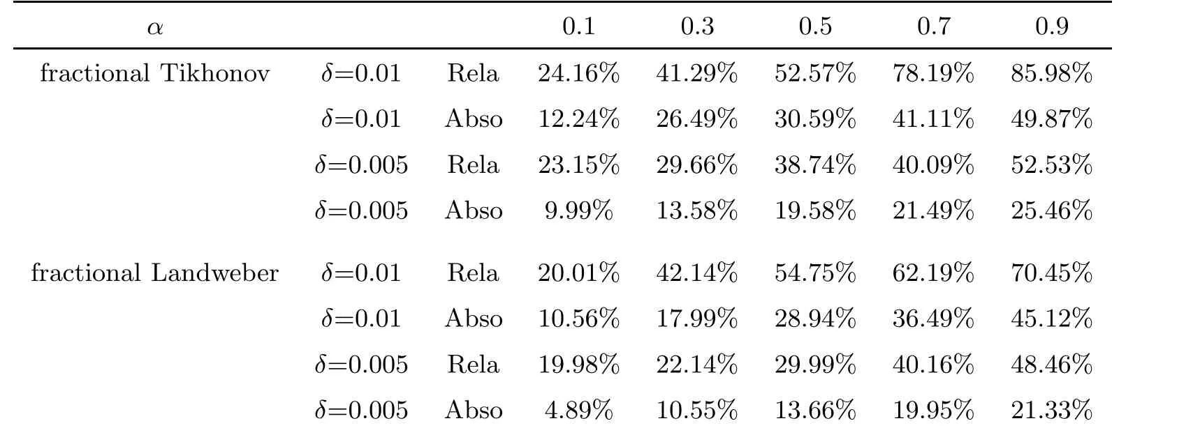
Table 6 Error behaviour of Example 3 for different α with δ =0.01,0.005
8 Conclusion
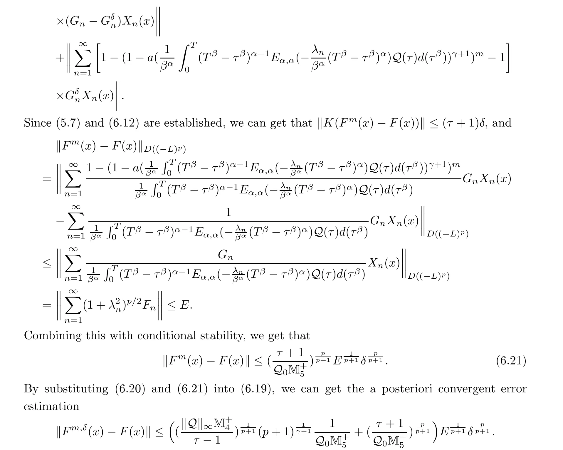
An inverse problem of identifying the source term for the time-fractional diffusion equation with a caputo-like counterpart hyper-Bessel operator has been considered. Based on an optimal error bound and conditional stability, we proposed the fractional Tikhonov regularization method and the fractional Landweber iterative regularization method for dealing with things and derived the a priori and a posteriori convergent estimates under a selection of a priori and a posteriori regular parameters. We find that the fractional Tikhonov regularization method has a saturation effect, while the fractional Landweber iterative regularization method has no saturation effect. For the fractional Tikhonov regularization method,the a priori error estimate is the best order for the optimal bound theorem when 0 <p <γ+1, and the a posteriori error estimate is optimal order when 0 <p <γ. However,for the Landweber regularization method,the a priori and the a posteriori error estimates are equally good for all p >0. Finally, numerical examples verify that the fractional Tikhonov regularization method and the fractional Landweber iterative regular method are efficient and accurate for recovering the stability of the inverse problem.
 Acta Mathematica Scientia(English Series)2022年4期
- Acta Mathematica Scientia(English Series)的其它文章
- ITERATIVE ALGORITHMS FOR SYSTEM OF VARIATIONAL INCLUSIONS IN HADAMARD MANIFOLDS*
- Time analyticity for the heat equation on gradient shrinking Ricci solitons
- The metric generalized inverse and its single-value selection in the pricing of contingent claims in an incomplete financial market
- The global combined quasi-neutral and zero-electron-mass limit of non-isentropic Euler-Poisson systems
- Some further results for holomorphic maps on parabolic Riemann surfaces
- Global well-posedness of the 2D Boussinesq equations with partial dissipation