Numerical Simulation of Space Fractional Order Schnakenberg Model
2021-06-22 04:21:30BANTingting班亭亭WANGYulan王玉蘭
BAN Tingting(班亭亭), WANG Yulan(王玉蘭)
College of Science, Inner Mongolia University of Technology, Hohhot 010051, China
Abstract: A numerical solution of a fractional-order reaction-diffusion model is discussed. With the development of fractional-order differential equations, Schnakenberg model becomes more and more important. However, there are few researches on numerical simulation of Schnakenberg model with spatial fractional order. It is also important to find a simple and effective numerical method. In this paper, the Schnakenberg model is numerically simulated by Fourier spectral method. The Fourier transform is applied to transforming the partial differential equation into ordinary differential equation in space, and the fourth order Runge-Kutta method is used to solve the ordinary differential equation to obtain the numerical solution from the perspective of time. Simulation results show the effectiveness of the proposed method.
Key words: Schnakenberg model; Fourier spectral method; numerical simulation; fourth-order Runge Kutta
Introduction
Fractional calculus was introduced in Newton’s time and has become a very hot topic in various fields. In fact, in recent years, fractional partial differential equations (FPDEs) have played an important role in mathematics, physics, engineering, economics and other disciplines. A large number of models can be described by fractional space and time derivative. Since the fractional derivative of a function depends on the value of the function on the whole interval, it is suitable for describing the memory effect and modeling of a system with spatial and temporal long range interaction[1]. In addition, fractional reaction-diffusion systems (FRDS) have received extensive attention in the study of nonlinear phenomena in science and engineering disciplines. Fractional order model is the best way to describe it. The main purpose of this paper is to consider the famous Schnakenberg model, which has been applied in many aspects of biology[2-4](the systemic inflammatory response syndrome(SIRS) epidemiological model of morbidity,etc.) and chemistry[5-7](autocatalytic systems,etc.). Because of the nonlinear term in the model, many models cannot get exact solution, and it is difficult to get exact solution. However, there are many numerical methods for solving the model, such as variational iteration method(VIM)[8-9], homotopy perturbation method (HPM)[10-12], He-Laplace Method[13], two-scale fractal derivative[14-15], barycentric interpolation collocation method(BICM)[16-17], and reproducing kernel method(RKM)[18-20]. But finding a simple and effective method is difficult. To solve this problem, we propose the Fourier spectral method, which has advantages in calculation precision, calculation amount and stability. The integer order Schnakenberg model is analyzed and discussed. In addition, we also simulate the fractional order case and give the simulation results. In Ref. [4], the fractional Schnakenberg model is given as
(1)
wherec1,c2,c3andc4are diffusion coefficients,γis constant,Ωis bounded inR2, and 1<α≤2. And initial conditions areu(x,y,0)=u0(x,y)andv(x,y,0)=v0(x,y). In particular, whenα=2, it is the standard Schnakenberg model.
In this paper, we numerically simulate (1) by using Fourier spectral method. The framework of this article is as follows. In section 1, we introduce the basics of fractional calculus. In section 2, we introduce the Fourier spectral method. In section 3, we simulate the model numerically. In section 4, we give the conclusions.
1 Basics of Fractional Calculus
There are several definitions of a fractional derivative of orderα>0, for instance, Riemann-Liouville, Caputo Riesz and Jumarie’s fractional derivative. Here, some basic definitions and properties of the fractional calculus theory which can be used in this paper are presented.
Defifinition1A real functionf(x),x>0 is said to be in the spaceCμ;μ∈Rif there exists a real numberp>μsuch thatf(x)=xpf1(x), wheref1(x)∈[0, ∞).Clearly,Cμ?Cβifβ≤μ.

(2)
where,mis the smallest integer which is larger than the parameterq,qis the order of the derivative and is allowed to be real or even complex, andais the initial value of functionf. In the present work only real and positive values ofqare considered.
2 Fourier Spectral Method
The Fourier transform and its inverse transform are defined as
(3)
(4)
It is easy to knowu(x)=F-1{F[u(x)]}.
Noting
(5)
For system formula (1) using Fourier transform, we can get
(6)
Using the fourth-order Runge Kutta to solve Eq. (6), we get the solution of system formula (1).
3 Numerical Simulation

Next, we simulate the space fractional order Schnakenberg model atα=2.0,α=1.6 andα=1.2 that simulates the initial conditions given by the homogeneous Neumman boundary conditions, and the results are shown as follows.
Case1Whenα=2,c1=c2=1,c3=c4=10,a=0.126 779,b=0.792 366 andγ=1 000, initial conditions


Fig. 1 Numerical solution of u in Case 1 at T=1
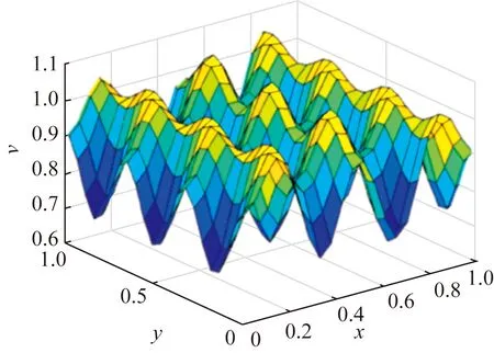
Fig. 2 Numerical solution of v in Case 1 at T=1
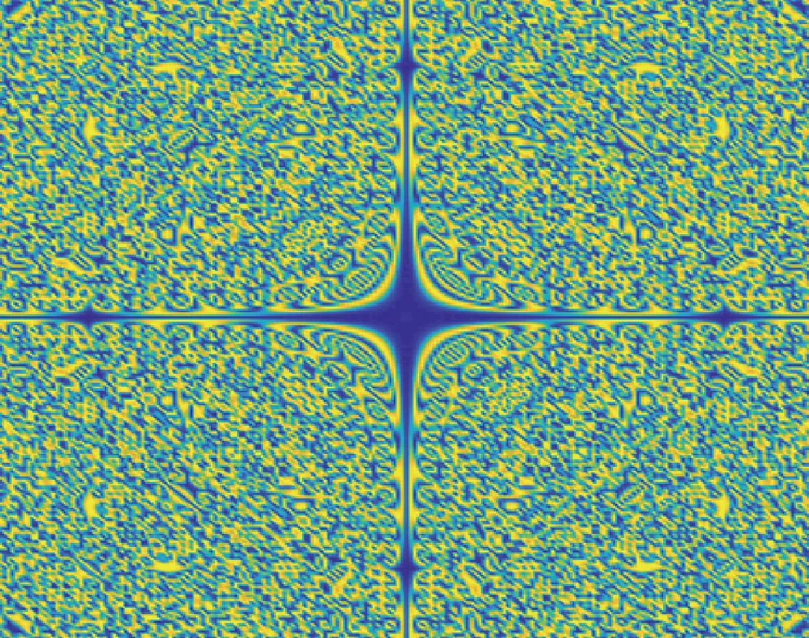
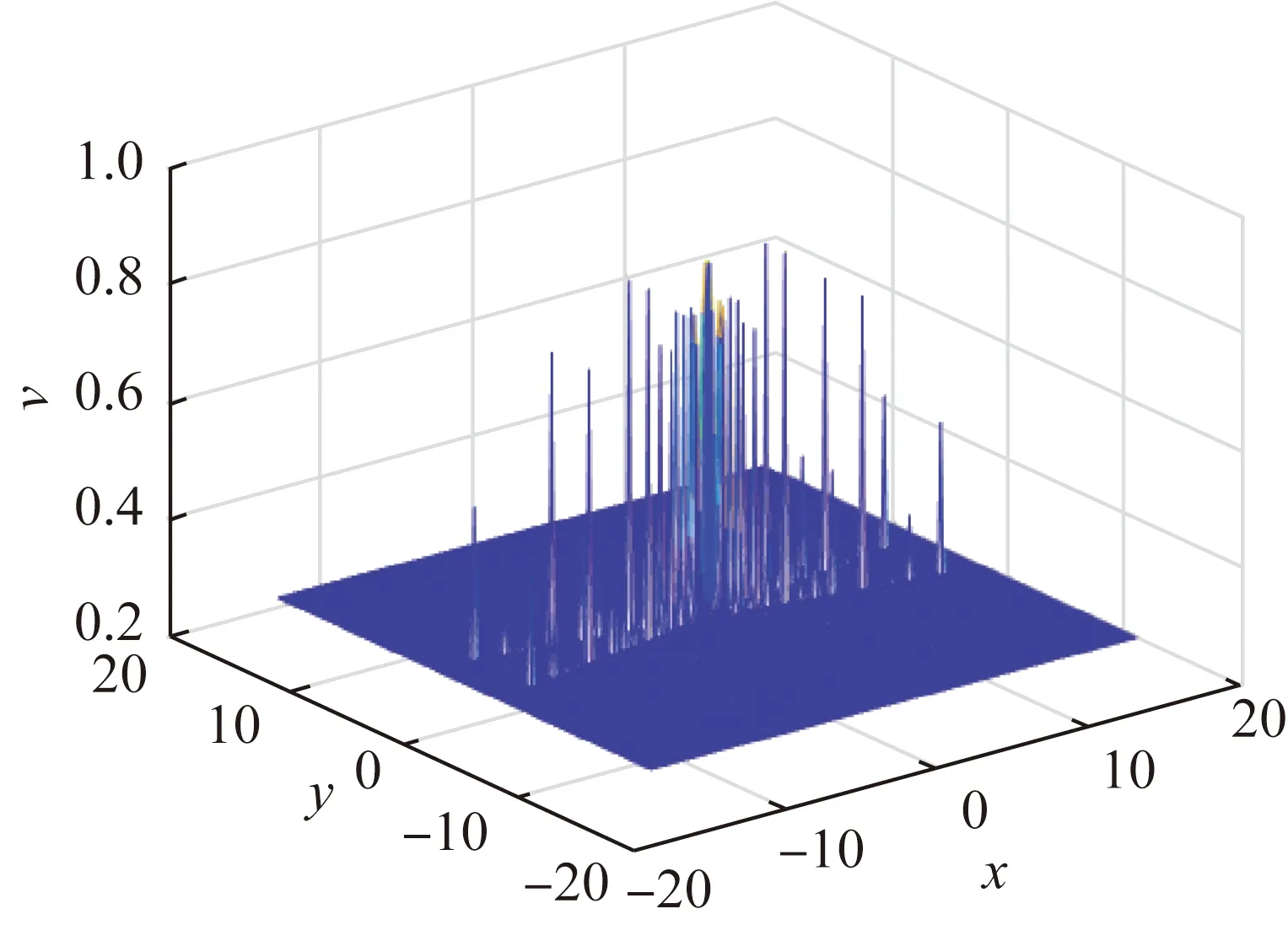
Case2Whenα=1.6,c1=0.05,c2=0.30,c3=0.15,c4=0.05,a=0.130 5,b=0.769 5,γ=1.5 and initial conditions areu=cos[sin(y2x2)],v=[0.769 5/(0.130 5+0.769 5)2]I, whereIis identity matrix. The simulation results are shown in Figs. 3-6.

(a) Numerical solution of u

(a) Numerical solution of v
(a) T=0.2, Ω = [-4, 4]
(a) T =0.2, Ω = [-4, 4]
We can know Figs. 3-4 simulates the numerical solution and pattern atT=0.2. Figures 5-6 describe the change of corresponding pattern with different interval length ofuandv, respectively.
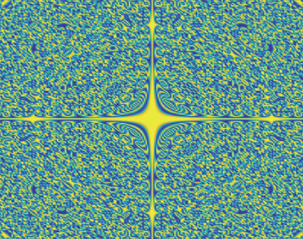
Case3Whenα=1.2,c1=0.05,c2=0.30,c3=0.05,c4=0.15,a=0.1,b=0.7,γ=1.5 and initial conditions areu=I+sech(x2/0.02-9+2y/0.01),v=sech(x2/0.02-0.5πy2/0.01), whereIis identity matrix. The simulation results are shown in Figs. 7-10.
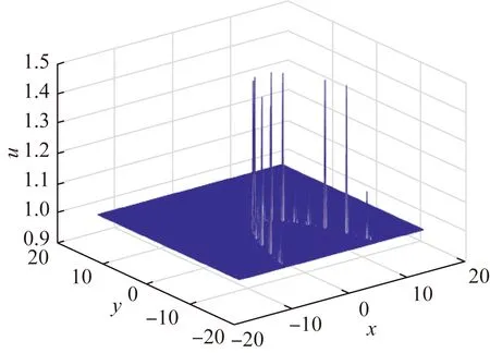
(a) Numerical solution of u
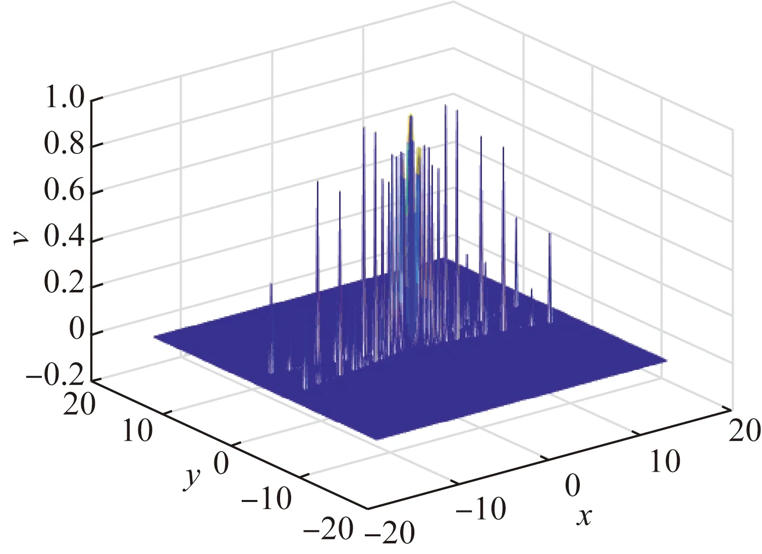
(a) Numerical solution of v
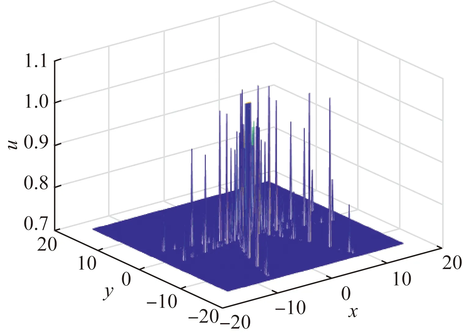
(a) Numerical solution of u
(a) Numerical solutions of v
We can know that Figs. 7-8 simulate the numerical solution and pattern atT=0, and Figs. 9-10 simulate the numerical solution and pattern atT=0.3. We can see the change of numerical solution and pattern with time.
4 Conclusions
This paper presents a Fourier spectral method for solving the space fractional order Schnakenberg model. Numerical simulation shows that the numerical results are consistent with the general theory, and the effectiveness of the proposed method is illustrated.
 Journal of Donghua University(English Edition)2021年2期
- Journal of Donghua University(English Edition)的其它文章
- Rational Design of a High-Performance KMnO4-Fe(Ⅱ)-Si Coagulant for Dye Removal
- Advances in Electrospun Nanofiber Yarns
- Thermal Insulation Properties of Microfibrillated Cellulose Aerogel
- Mechanical and Thermal Properties of Apocynum and Ramie Fiber Mat Reinforced Polylactic Acid Composites
- Symmetry Classification of Partial Differential Equations Based on Wu’s Method
- Meta-Analysis on the associations between Prenatal Perfluoroalkyl Substances Exposure and Adverse Birth Outcomes