Closed form soliton solutions of three nonlinear fractional models through proposed improved Kudryashov method

Zillur Rahman, M Zulfikar Ali, and Harun-Or Roshid

1Department of Mathematics,Comilla University,Cumilla-3506,Bangladesh

2Department of Mathematics,Rajshahi University,Rajshahi-6205,Bangladesh

3Department of Mathematics,Pabna University of Science and Technology,Pabna-6600,Bangladesh

Keywords: improved Kudryashov method,fractional electrical transmission line equation,fractional nonlinear complex Schr¨odinger equation,M-fractional Schr¨odinger–Hirota(s-tM-fSH)

1. Introduction

The accurate modeling of nonlinear phenomena related to natural happening is really impossible without fractional derivatives. Nowadays, the fractional calculus has been frequently used to model the nonlinear systems in various fields such as neuron networks,[1]dust acoustic and dense electron–positron–ion wave,[2]plasma physics,[3]quantum mechanics,[4]nonlinear optical fiber communication,[5]superconductivity and Bose–Einstein condensates,[6]electrics signal processing,[7]biological dynamics,[8]water wave dynamics,[9]electro–magnetic waves,[10]nonlinear electrictransmission line,[11]and many other areas. Various types of exact solutions including periodic wave and solitons are essential to realize intrinsic dynamical structure of such models even universe. Up to now, huge improvements have been achieved in the development of techniques to evaluate such exact solutions of the nonlinear models. Several powerful methods are as follows. The exp(?Φ(η))-expansion,[12]Hirota bilinear,[13]B¨aklund transformations,[14]modified simple equation,[15]tanh method,[16]tan(Θ/2)-expansion,[17]soliton ansatz,[18,19]auxiliary equation,[20]sine-cosine,[21]homogeneous balance,[22]Jacobi elliptic function expansion,[23](G′/G)-expansion,[23,24]modified double sub-equation,[25]exp-function,[26]generalized Kudryashov[26]methods, and many others. It should be pointed out that all the mentioned approaches have some advantages and also a few disadvantages to integrate complex nonlinear systems. As is well known, no approach is suitable for all equations. Thus, we are willing to propose a new and active approach namely improved Kudryashov method (IKM) on the basis of the generalized Kudryashov method[26]by changing its auxiliary equations.

Now,we come to shed light on the nonlinear space–time fractional electrical transmission lines (s-tfETL),[11,27]the time fractional complex Schr¨odinger (tcFSE),[28]and space–time M-fractional Schr¨odinger–Hirota (s-tM-fSH)[29]models via the proposed IKM. These models have been widely studied in many aspects for the non-fractional differential case. Abdou and Soliman[11]only solved the fractional transmission line equation thru the generalized exp(??(ξ))-expansion and generalized Kudryashov methods. But nonfractional transmission line equation has been studied by Zayed and Alurrfi[30]thru using new Jacobi function expansion method,by Kumar et al.[31]thru using three schemes as modified Kudryashaov,Sine–Gordon-,and extended Sinh–Gordonexpansion methods, and by Shahoot et al.[32]thru using the(G′/G)-expansion scheme. Besides, the time fractional complex Schr¨odinger equation(FSE)is a vital nonlinear model in solitonic field. The model describes the collision of the adjacent particles of identical mass on a lattice structure through a crystal and demonstrate the fundamental properties of string dynamics with fixed curvature space.[13]This model was first developed by Laskin[33]which occurs in many important areas as water wave, fluid dynamics, bio-chemistry, optical pulses propagation into nonlinear fiber, and plasma physics. Few researchers made much more effort to investigate the complex fractional Schr¨odinger model: Khater[34]studied it by a supplementary equation as well as (G′/G)-schemes, Alam and Li[28]presented wave solutions through modified(G′/G)-expansion technique. In recent years, Sousa and Oliveira invented an M-fractional order derivative.[35]So, we also considered another model namely the space–time truncated M-fractional Schr¨odinger–Hirota model[29]which frequently arises in quantum Hall effect, optical fibers, heat pulses in solids,and more areas. Sulaiman et al.[29]investigated the Mfractional SH model to present optical soliton solutions with the help of a sinh-Gordon technique. But non-fractional SHE is investigated.[36,37]

This research is intended to execute the improved Kudryashov technique to determine abundant exact solitonic solutions as periodic envelope,exponentially changeable soliton envelope, rational, combo periodic-soliton, and combo rational-solitonic solutions of the s-tfETL,[11,27]the tfcSE,[28]and the s-tM-fSH[29]models, which take an essential part in nonlinear complex phenomena of physical sciences.

2. Conformable M-fractional and fractional derivatives with properties

The new M-fractional derivatives are given below.[35]

Let ?:[0,∞)→?, then M-fractional derivative ?with order α can be written as follows:

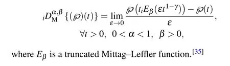
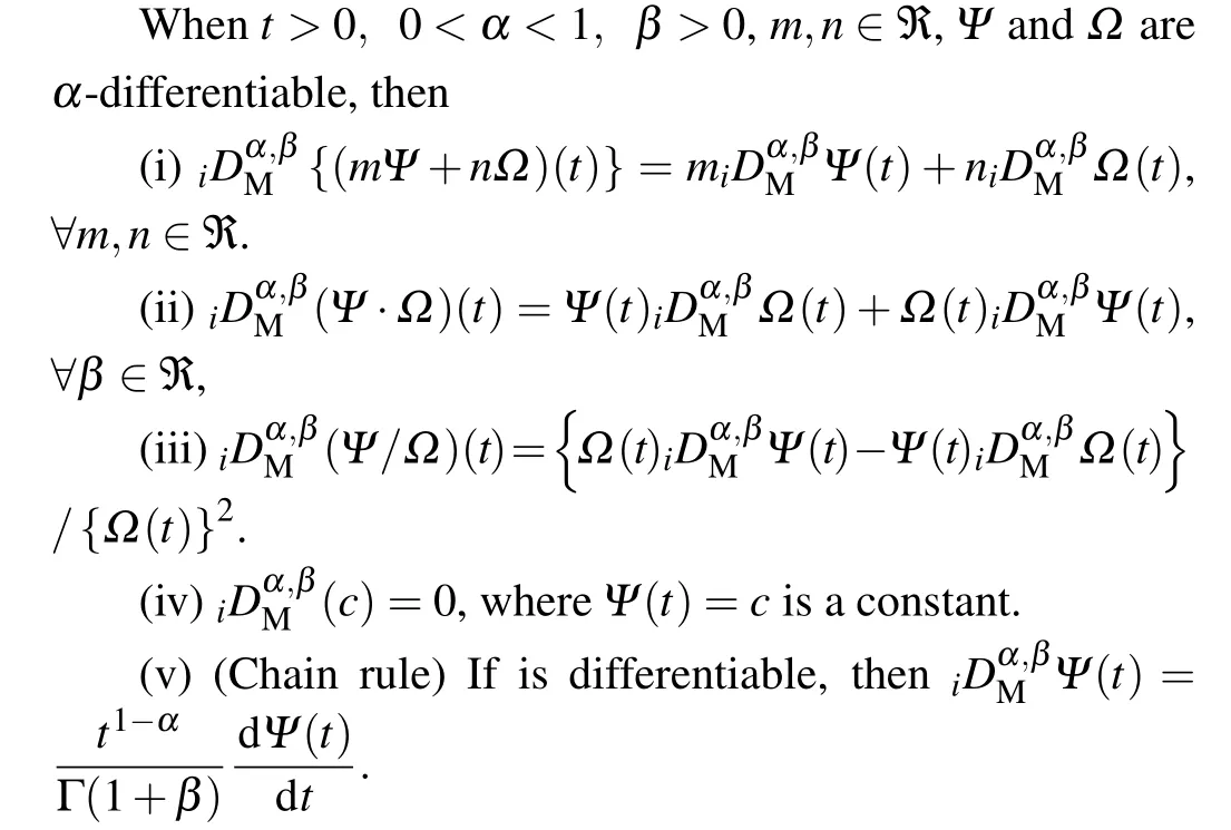
2.1. Properties of new M-fractional derivatives

If a function defined by ? :(0,∞)→?,the conformable fractional derivative with order υ is defined[38]as

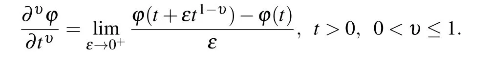
2.2. Properties of conformable fractional derivative

3. Algorithm of proposed method

The fundamental phases of the technique are as follows.

Step 1 At first,let the subsequent fractional equation with the variables x and t be

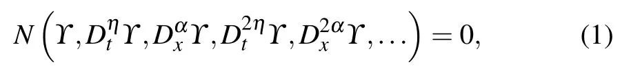
where the function ? =?(x,t) is an unknown wave surface,and N is a function of ?(x,t) and its highest order fractional derivatives.

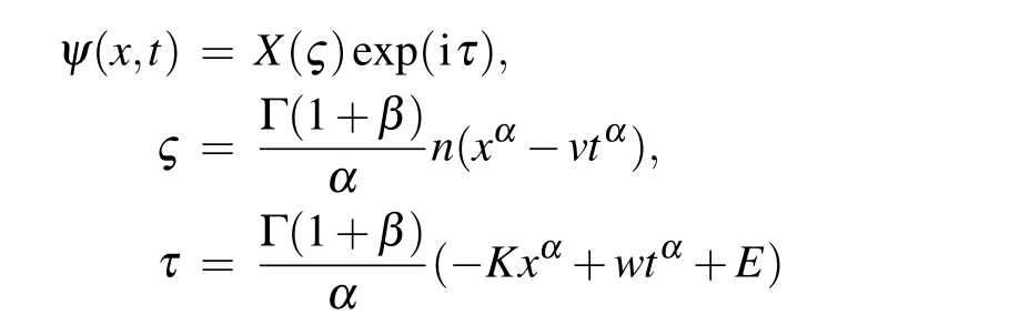
Step 2 For complex nonlinear model, take the transformation ?(x,t)=?(ζ)exp(iτ) with travelling wave variables for space–time fractional model

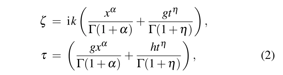
and for no complex model,adopt the transformation ?(x,t)=?(ζ) and travelling wave variable for space–time fractional model

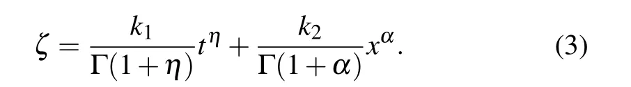
Substituting the above Eq. (2) or Eq. (3) into Eq. (1), the resulting equation is reduced to an ordinary differential equation(ODE)with the help of fractional complex transformation producing

then equation(1)turned into the following form,

The prime of ?indicates the usual meaning of derivative.

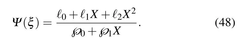
Step 3 Picking a trial solution for Eq.(5),that is,

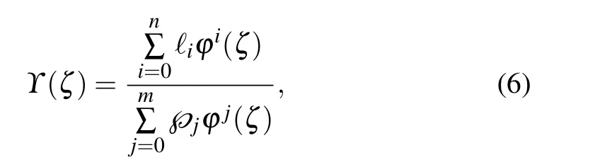
where ?iand?jare the real fixed values,and n ＞0 and m ＞0 are integers with the restraint ?n,?m/=0.

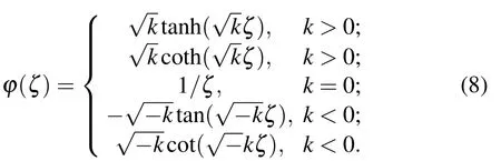
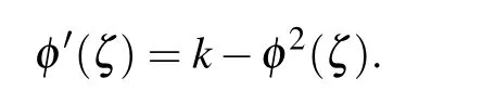
Here, we just need to take a different auxiliary equation which is satisfied by ?(ζ)and expressed as

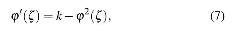
where k is an arbitrary constant. Some special solutions of the Riccati equation,i.e.,Eq.(7),are given by

Step 4 Combining Eqs.(5),(6),and(7)through computational software,we can get polynomial in ?(ζ).Taking each of coefficients of ?κ(ζ)(κ =0,1,2,3...)to be zero and thus some equations are formed in-terms of unknown constants ?κand ?κ. Solving these unknown constants then putting them into a trial solution together with the solutions Eq.(8),the exact solution of Eq.(1)is obtained.

Remark 1 It is noted that the auxiliary equation in the generalized Kudryashov[11,26]and the modified Kudryashov schemes[31]each are capable to provide only one solution in terms of exponential function. Consequently, the auxiliary Eq. (7) in the proposed IK scheme degenerates five different solutions involving hyperbolic, rational, and trigonometric functions. In the concluding remark, we can say that the introduced scheme will be more useful than the other exiting schemes for different types of solutions.[26,31]

Remark 2 The proposed technique is easier as it takes less calculations than the modified (G′/G)-expansion technique.[28]It is noticed that the modified(G′/G)-expansion method takes double auxiliary equations while we consider only Riccati equation as an auxiliary equation.

4. Applications

4.1. Spatiotemporal fractional electrical transmission line equation(s-tfETLE)

General form of s-tfETLE can be written as follows:[11]

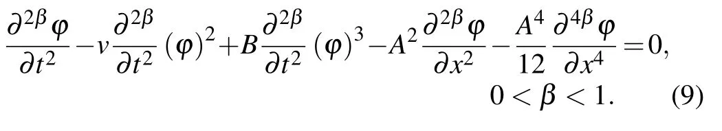
The s-tfETL equation(9)is one of the important equations in fractional electrical physics.The equation describes data communication and is modified in a telecommunication system.

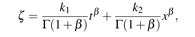
Considering ?(x,t)=φ(ζ) and this nonlinear s-tfETL partial evolution model can be converted into a nonlinear integer order ordinary differential ETL as follows:

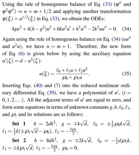
As is well known, the delicate balance between the height derivative and height nonlinear terms gives n=m+1. Consider a trial solution Eq.(6)in the following form(m=1,?n=2):

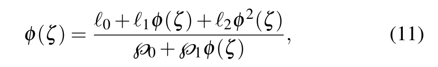
where the auxiliary equation is used

Inserting Eq.(11)with Eq.(7)into the reduced nonlinear ordinary differential Eq. (10), we have a polynomial of φi,(i=0,1,2,...). All the adjacent terms of φiare equal to zero,and form some equations in terms of unknown constants?0,?1,?2,?0,?1,k1, and k2. Solving the equations via Maple software,we obtain the five sets of solutions for L=Γ(1+β).

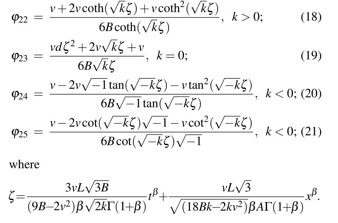
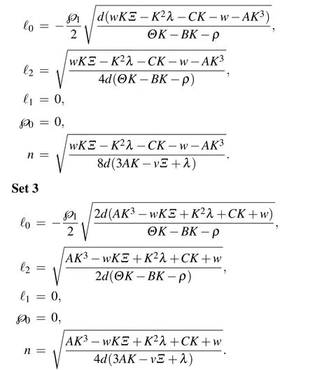
The general solutions of s-tfETL equations for solution Set 3 are

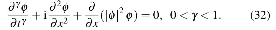
4.2. Time fractional complex Schro¨dinger equation(tfcSE)

The section starts with the tfcSE in the form[31,32]

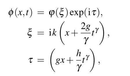
For the purpose of mathematical conversion, bring the transformations:and it converts this tfcSE to the one without fractional-order nonlinear SE:

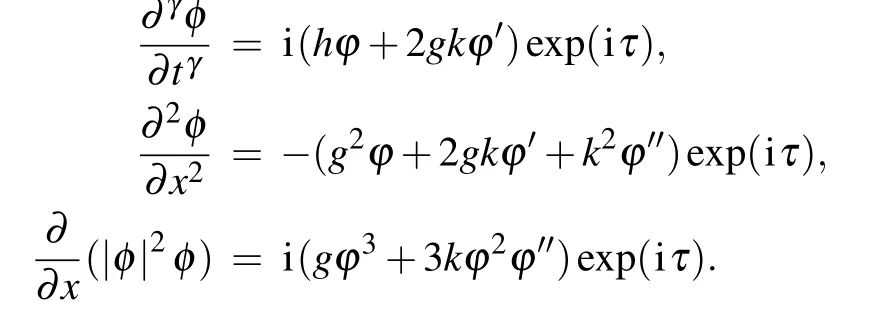
We obtain the nonlinear complex PSE by using the above expression,

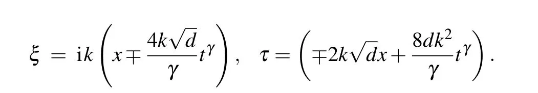
For Set 1, the solution sets of the considered equation hold: for d ＞0,we have

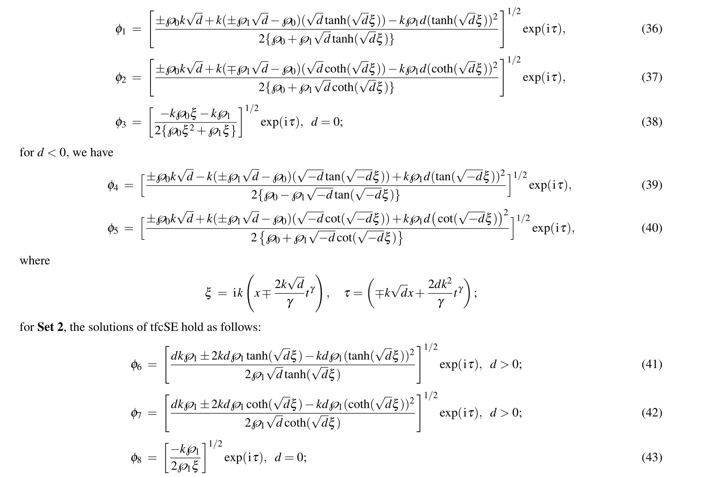
where

4.3. M-fractional Schro¨dinger–Hirota equation (s-tMfSH)

This subsection starts with the Schr¨odinger–Hirota equation[35]with the form

where ψ(x,t)is a complex function, coefficients Θ, λ, Ξ, A,and C are the self-steepening,group velocity,spatiotemporal,3rd dispersion,and inter-modal dispersion terms respectively.Parameters B and ? are nonlinear dispersions.

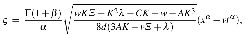
Substituting the complex wave transformation

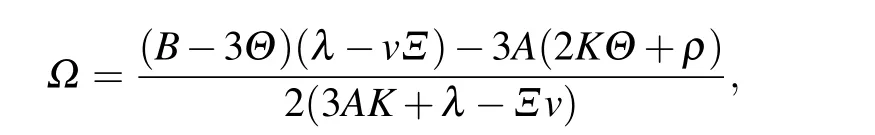
into Eq.(46),we attain to the ODE with two conditions:

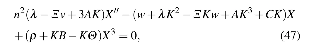
with

The homogenous balance provides n=m+1. For m=1,we have n=2. So equation(6)reduces to the following equation by using X′(ζ)=d ?X2(ζ),

Inserting Eq. (48) and Eq. (7) into the reduced nonlinear ordinary differential equation (47), we have a polynomial of Xk,(k=0,1,2,...). All the adjacent terms of Xkare equal to zero,and form some equations with unknown constants ?0,?1,?2,?0,?1,and n. Solving the equations with Maple software,we get three sets of solutions:

Set 1

Set 2

For Set 1, the solutions of spatiotemporal M-fractional SH equation hold:

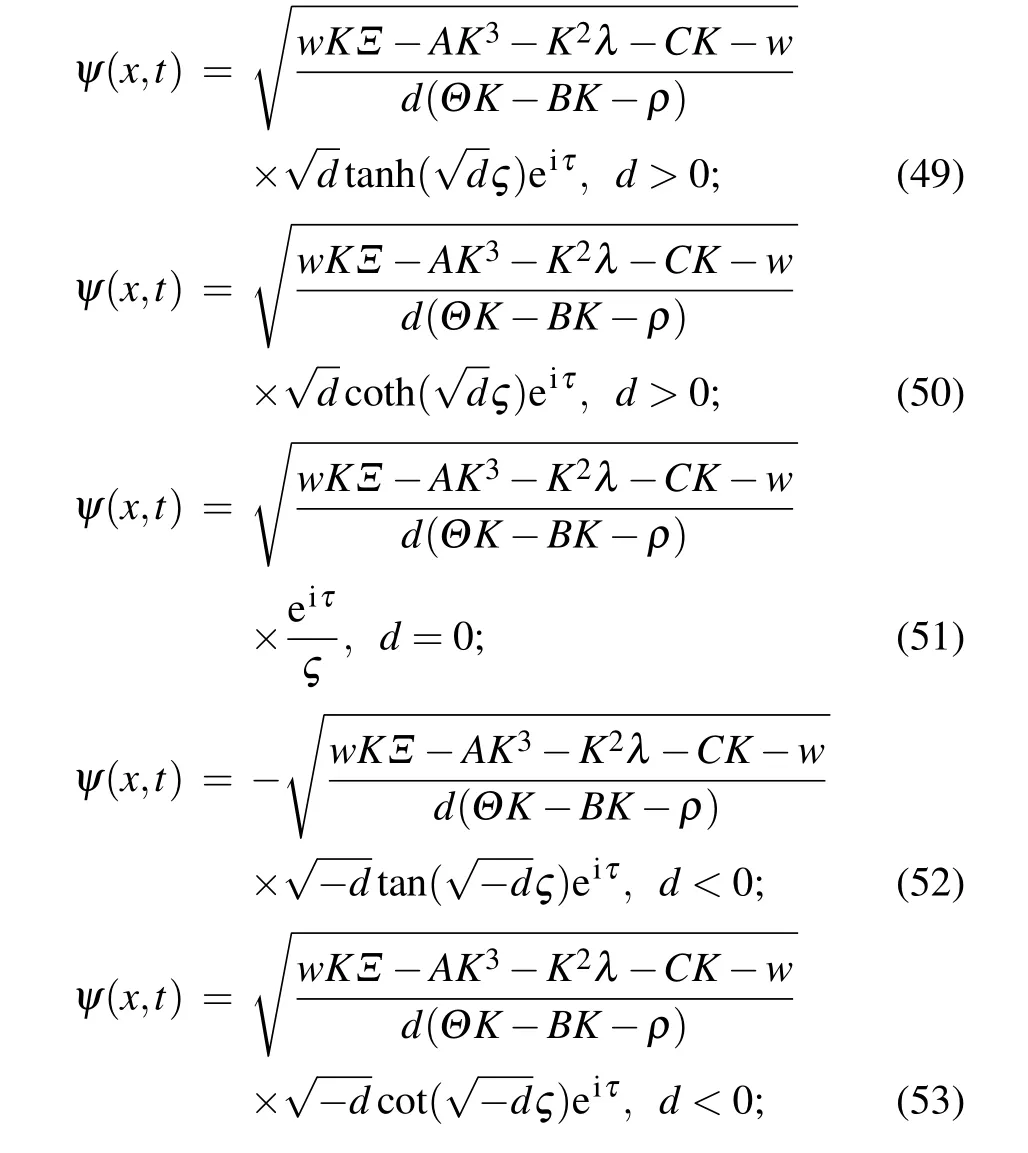
where

For Set 2, the solutions of spatiotemporal M-fractional SH model hold:

where

For Set 3, the solutions of spatiotemporal M-fractional SH equation hold:

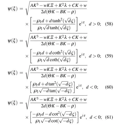
where

5. Graphical representations

5.1. Graphical representation of solutions for stFETL model

The research findings are in the types of hyperbolic,rational, and trigonometric functions. All the results are analyzed and some of them have shown graphically in Figs.1–3.

5.2. Graphical representations of solutions for tfcSE

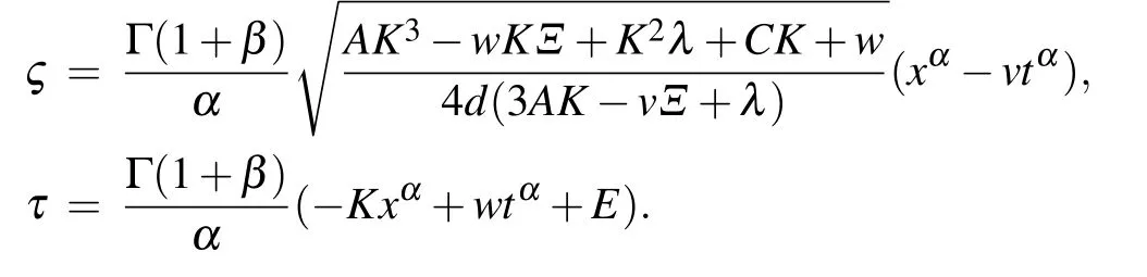
Two sets of results are found in the study of the tfcSE.We analyze all results. Five results are graphically shown Figs.4–7. The three-dimensional(3D)contour, and two-dimensional(2D)plots show the changes of amplitudes,directions,shapes of wave as well as the nature of the solitary waves of gained solutions in space x with time t below.

5.3. Graphical representations of solutions for s-tM-fSH

The derived results are in a variety of hyperbolic,rational,and trigonometric functions. All of the results are analyzed and some of them are shown graphically in Figs.8–13,where the patterns and natures of the wave surfaces are shown clearly with 3D,2D,and contour plots.

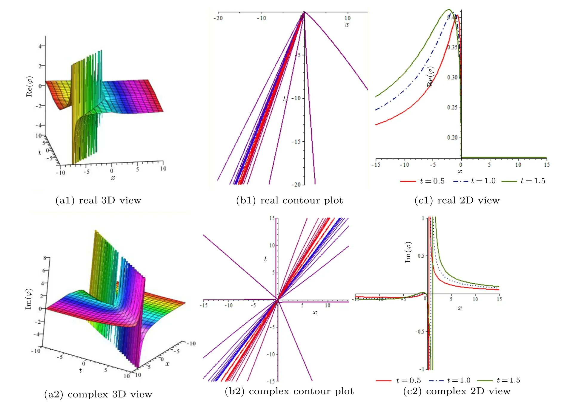
Fig.1. (a),(b)Real and complex three-dimensional(3D)surface and contour plot of solution ?(x,t)of Eq.(12)for k=2,β =0.1,v=0.5,A=1,and B=?1,and(c)two-dimensional(2D)plot for t=0.5,1 and 1.5 with parametric values above.

Fig. 2. (a), (b) Periodic rogue waves from real and complex 3D surface and contour plot of solution ?(x,t) of Eq. (15) for k=?2, β =1, v=0.5,A=1,and B=?1,and(c)2D plot for t=0.5,1.25,and 2.25 with parametric values above.

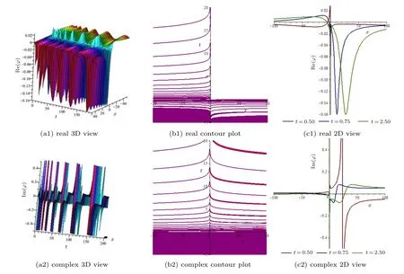
Fig.3. (a), (b)Real and complex 3D surface and contour plot of solution ?(x,t)of Eq.(30)for k=?2, β =0.1, ?2 =1, v=3, A=2, B=?1, and k2=2,and(c)2D plot for t=0.5,0.75,and 2.5 with parametric values above.

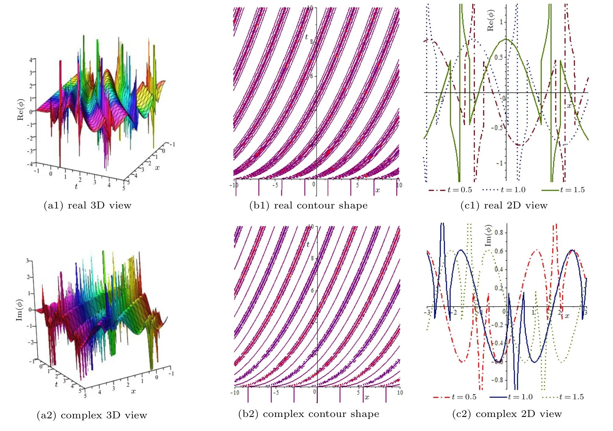
Fig.4. Solitonic solution φ(x,t)of Eq.(36)for d=2,?1=0.5,?0=1,γ =0.5,and k=0.8 and t=0.5,1,and 1.5 for 2D graph.

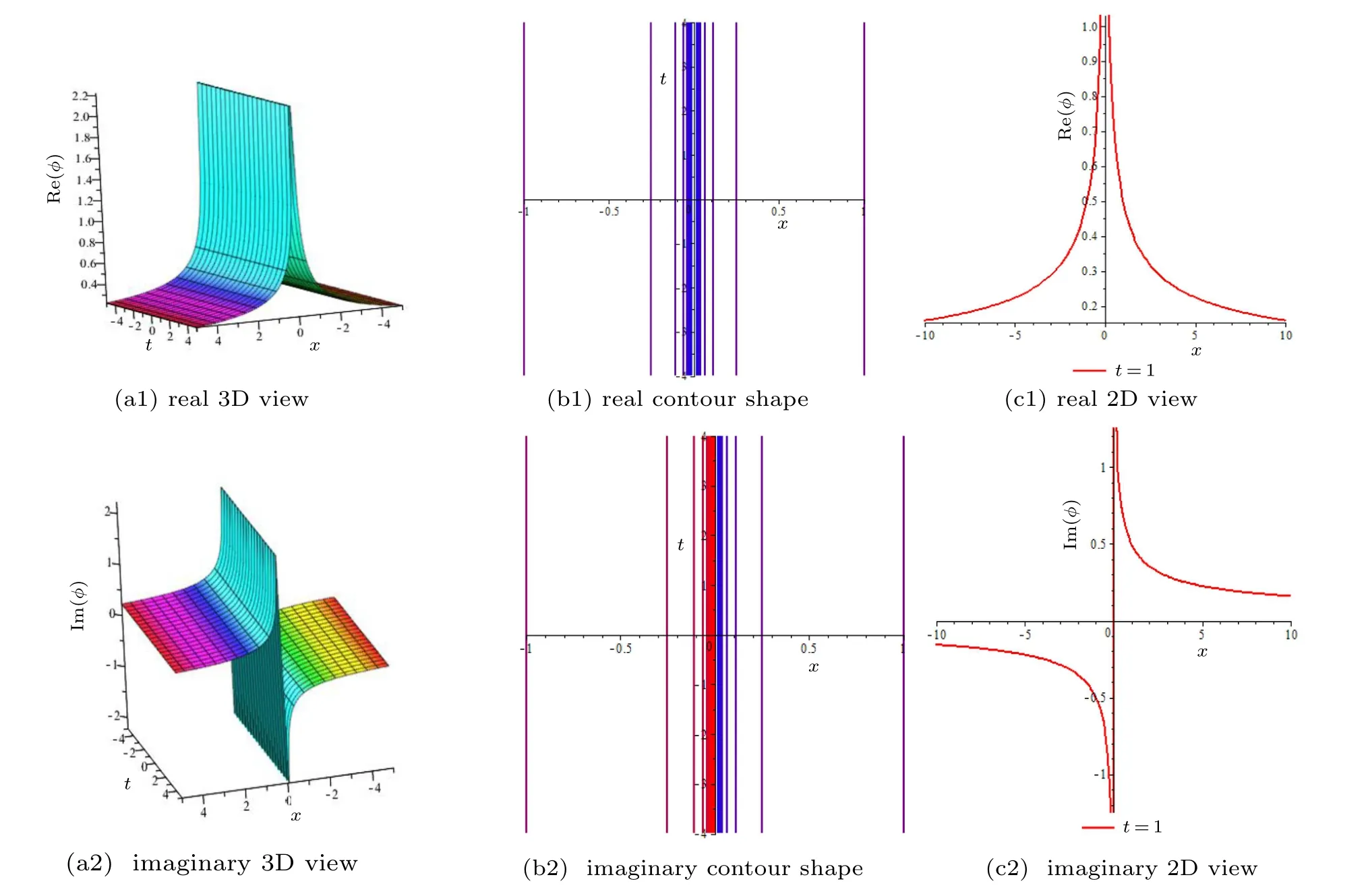
Fig.5. Plot of solitonic solution φ(x,t)of Eq.(38)for d=0,?1=2,?0=1,γ =2/3,and k=0.8 and t=1 for 2D graph.

Fig.6. Solitonic solution φ(x,t)of Eq.(39)for d=?2,?1=2,?0=1,γ =4/5,and k=1 and t=0.1,0.8,and 1.5 for 2D graph.

Fig.7. Solitonic solution φ(x,t)of Eq.(42)for d=2,?1=0.5,?0=1,γ =0.5,and k=0.8 and t=0.1,1,and 2 for 2D graph.

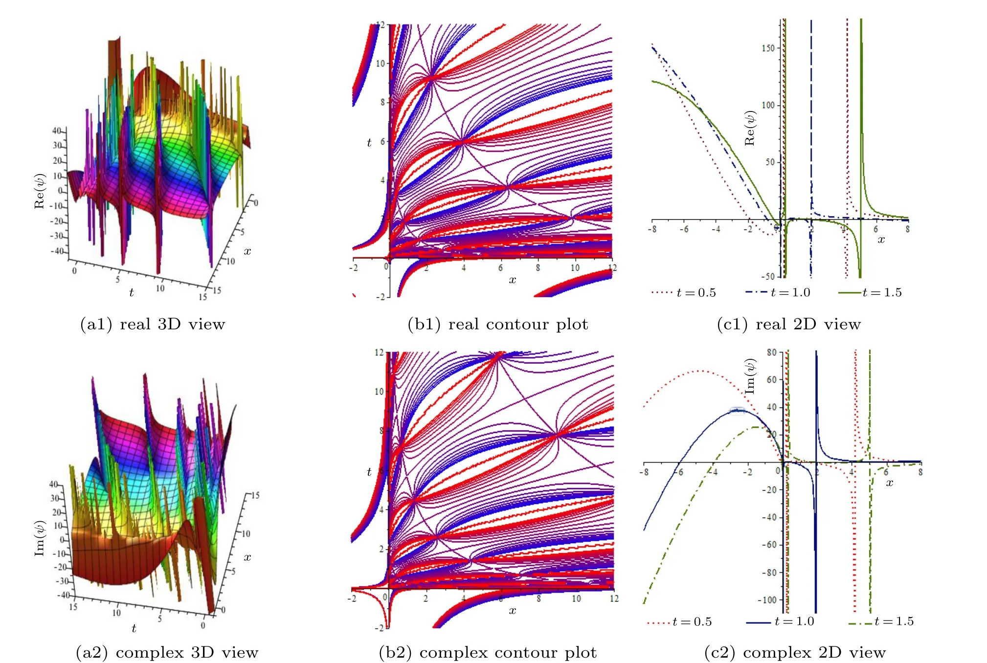
Fig.8. Solitary wave solution ψ(x,t)of Eq.(49)for d=2,α =β =0.25,A=K=λ =Θ =σ =1,w=?1,ρ =2,Ξ =2,ν =3,E=6,and t=0.5,1,and 1.5 for 2D graph.

Fig.9. Solitonic solution ψ(x,t)of Eq.(52)for d=?2,α=0.5,β =B=0.75,A=2,K=5,w=?1,Θ =3,ρ=1,Ξ =4,ν=1,λ =1,E=6,and σ =3 and t=1,1.5,and 2 for 2D graphs.

Fig.10. Solitonic solution ψ(x,t)of Eq.(54)for α =0/3,β =B=0.5,A=1,K=1,w=?1,Θ =1,ρ =2,Ξ =2,ν =0,λ =1,and E=6 and for 2D graph t=0.5,1,and 1.5.

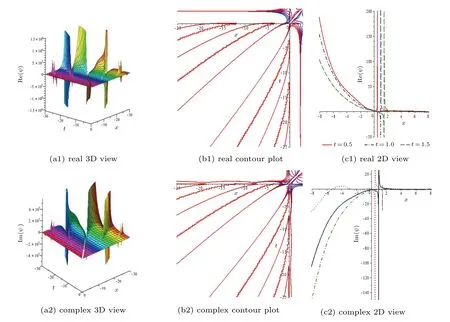
Fig.11. Wave solution ψ(x,t)of Eq.(56)for α =β =B=0.5, A=1, K =1, w=?1,Θ =1, ρ =1, Ξ =2, ν =1, λ =1, and E =6, and for 2D graph t=0.5,1,and 10.5.

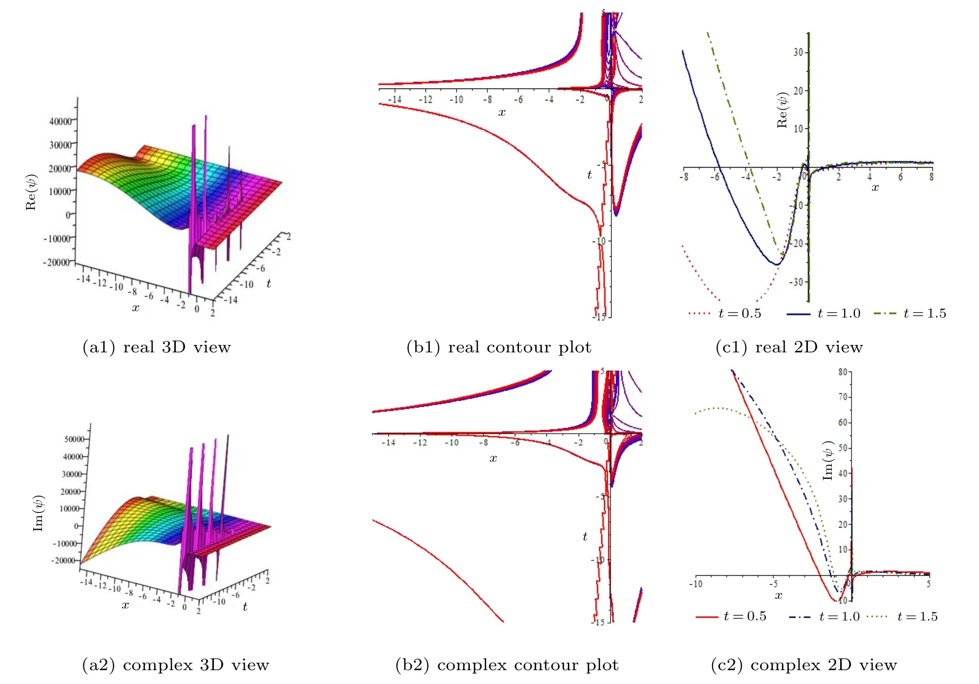
Fig.12. Wave solution ψ(x,t)of Eq.(59)for α =β =B=0.25,A=1,K=1,w=?1,Θ =1,ρ =Ξ =2,ν =0.5,λ =1,and E =6,and for 2D graph t=0.5,1,1.5.

Fig.13. Solution ψ(x,t)of Eq.(61)for d=2,α=β =B=0.25,A=K=1,w=?1,Θ =1,ρ=Ξ =2,ν=12,λ =1,and E=6,and for 2D graph,t=0.5,1,and 1.5.

6. Conclusions

In this work, we present an integral technique to solve fractional nonlinear differential models. To test the validity of the procedure,we solve three nonlinear fractional models: the s-tFETL(Figs.1–3), the tfcSE(Figs.4–7), and the s-tM-fSH(Figs. 8–13) models. The periodic envelope, exponentially changeable soliton envelope, rational rogue waves, periodic rogue waves, combo periodic-soliton, and combo rationalsoliton solutions are formally derived from the models. The achieved results show that the proposed technique is a very effective, concise, and robust mathematical tool in comparison with the generalized Kudryashov method and the modified Kudryashov method of solving other fractional nonlinear models.