Exact solution of the Gaudin model with Dzyaloshinsky–Moriya and Kaplan–Shekhtman–Entin–Wohlman–Aharony interactions*

Fa-Kai Wen(溫發楷) and Xin Zhang(張鑫)

1State Key Laboratory of Magnetic Resonance and Atomic and Molecular Physics,Wuhan Institute of Physics and Mathematics,Chinese Academy of Sciences,Wuhan 430071,China

2Fakult¨at f¨ur Mathematik und Naturwissenschaften,Bergische Universit¨at Wuppertal,42097 Wuppertal,Germany

Keywords: integrable models,Gaudin model,Bethe ansatz,Bethe states

1. Introduction

The Gaudin model is an important integrable system with long-range interaction.[1]It is closely related to the central spin model[2,3]and BCS model,[4–9]which has been widely used in the study of metallic nanoparticles,[10]quantum dots,[11]noisy spins,[12]Rydberg atoms,[13]and so on.Based on the exact solutions of the Gaudin model,its correlation functions,[14]quantum dynamics[15–18]and coherence[19]have always been the focus of research.

The Gaudin Hamiltonian can be constructed by taking the quasi-classical expansion of the transfer matrix of the spin chain.[20–24]For the periodic case, the corresponding Gaudin Hamiltonian includes the external field on the central spin(B)and Heisenberg exchange interaction(Ak). For the open case,the corresponding Gaudin Hamiltonian also includes the Dzyaloshinsky–Moriya (DM) interaction (Dk)[25,26]and the Kaplan–Shekhtman–Entin–Wohlman–Aharony(KSEA)interaction(Mk),[27,28]i.e.,

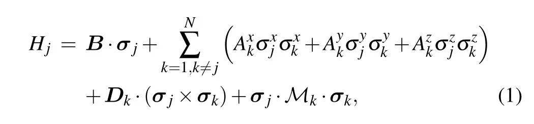
where N is the number of spins. The constants B, Ak,Dkand Mkare defined below and their values rely on the boundary parameters and a set of inhomogeneous parameters{θ1,...,θN}. For the generic open cases, the corresponding Gaudin Hamiltonian has no obvious reference state due to the U(1)symmetry breaking(i.e.,the total spin along z-direction is not conserved). This leads to employing the conventional Bethe ansatz methods to approach the eigenvalues and Bethe states of the model very involved. With the help of the offdiagonal Bethe ansatz(ODBA)method,[29,30]the eigenvalues of the XXX model with generic open boundaries were given in Ref. [31]. Recently, the Gaudin model has been revisited many times.[32–34]However, the Bethe states of the Gaudin Hamiltonian(1)are still absent.

In this paper, one of our aims is to construct the Bethe states of the Gaudin model (1). By employing some gauge transformations, we obtain the operators and reference state for constructing the Bethe states, respectively. Taking the quasi-classical expansion of the Bethe states of the spin chain,we obtain the Bethe states of the Gaudin model (1). We also study the degeneration of the Bethe states when the model recovers the U(1)symmetry.

The rest of this paper is organized as follows. In Section 2, we present the ODBA solutions of the Gaudin model.In Section 3, with the help of the ODBA solutions, we construct the Bethe states of the Gaudin model. The Bethe states,eigenvalues and Bethe ansatz equations recovering that of the Gaudin model with the U(1)symmetry are given in Section 4.We summarize our results and give some discussions in Section 5. Some technical proofs are given in Appendix A.

2. ODBA solutions

The integrability of the Gaudin model is associated with the R-matrix

where u is the spectral parameter and η is the crossing parameter. The R-matrix satisfies the quantum Yang–Baxter equation

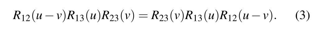
Here R21(u)=P12R12(u)P12with P12being the usual permutation operator. In what follows, we adopt the standard notations: for any matrix O ∈End(V),Okis an embedding operator in the tensor space V ?V ?···, which acts as O on the k-th space and as identity on the other factor spaces;Rkl(u)is an embedding operator of R-matrix in the tensor space,which acts as an identity on the factor spaces except for the k-th and l-th ones.[35]

The general reflection matrices are given by[31]

which satisfy the reflection equation(RE)

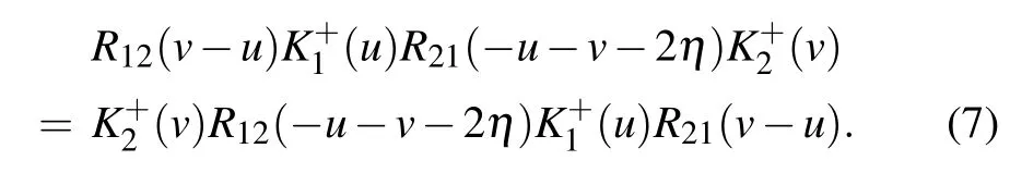
The dual K-matrix K+(u)is

which satisfies the dual RE

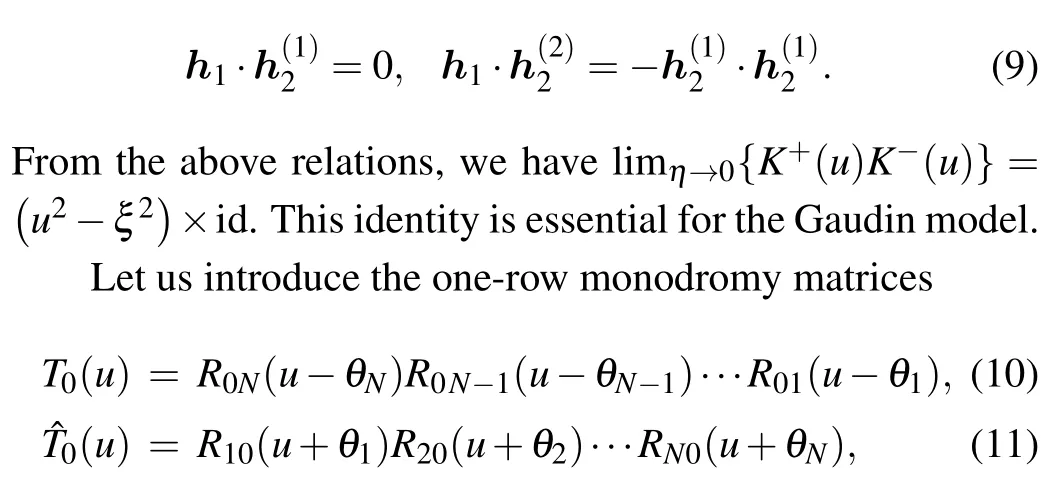
The parameters ˉξ and ?2depend on the crossing parameter η.Expansion of ˉξ and ?2with respect to η is as follows:

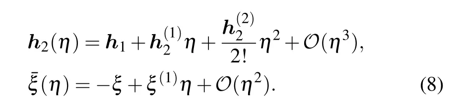
Using the normalization(6),we have

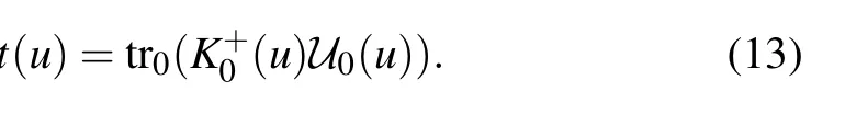
and the double-row monodromy matrix

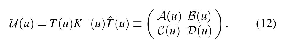
Then the transfer matrix is given by

With the same procedure introduced in Ref.[36],one can obtain the commutativity of the transfer matrix [t(u),t(v)]=0,which ensures the integrability of the model. Expanding the transfer matrix t(u) at the point u=θjaround η =0,[36]we obtain

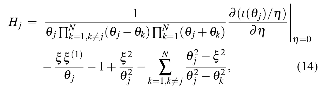
where the constants in the Hamiltonian (1) are expressed in terms of the boundary parameters in the corresponding Kmatrices given in Eqs.(4)and(6)as follows:

where the function Q(u) is parameterized by N parameters{λj|j=1,...,N}

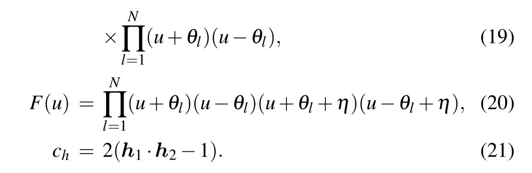
and the functions a(u), d(u), F(u) and the constant chare given by

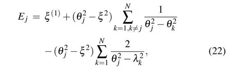
By using the relation(14),the energy Ejof the Gaudin Hamiltonian Hjcan be obtained,

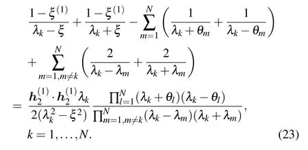
and the N Bethe roots{λk|k=1,...,N}should satisfy a set of Bethe ansatz equations(BAEs),

3. Bethe states of the Gaudin model

With the above relations,the transfer matrix t(u)can be rewritten as

Then, the boundary K?(u) matrix can be transformed into a lower triangular matrix

and an upper triangular matrix

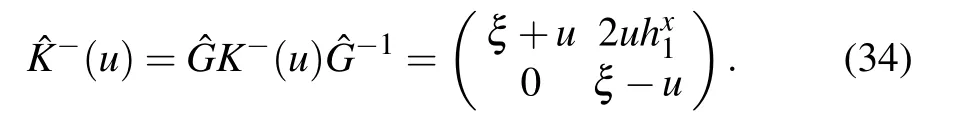
Here we use the following notations for the gauge transformed matrices: ?O=GOG?1, ˉO= ˉGOˉG?1and ?O= ?GO ?G?1,where O is an arbitrary matrix in the auxiliary space. With the gauge transformation matrices ˉG and ?G,we introduce the following new reference states:

Using a similar method in Ref.[37],we construct the left and right Bethe states of the inhomogeneous XXX Heisenberg spin chain with the generic open boundaries

The proofs are given in Appendix A.

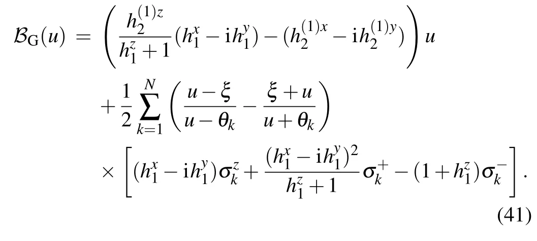
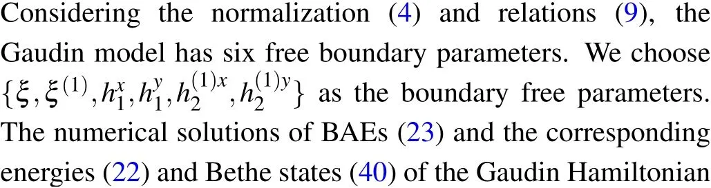
With the relation (14), the Bethe state of the inhomogeneous XXX Heisenberg spin chain can be expanded as[21]

Table 1. Solutions of BAEs (23) for the case of N = 3, j = 1, {θk} ={1.19,2.20,3.58}, ξ =0.8i, ξ(1) =1.2, =0.3, =0.5, h=0.2i,=0.7i. The symbol n indicates the number of the eigenvalues, =Hj|ψ〉?|ψ〉, and is the corresponding energy. The energy calculated from Eq.(22)is the same as that from the exact diagonalization of the Gaudin Hamiltonian(1).

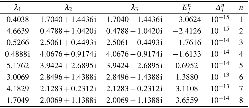
Table 1. Solutions of BAEs (23) for the case of N = 3, j = 1, {θk} ={1.19,2.20,3.58}, ξ =0.8i, ξ(1) =1.2, =0.3, =0.5, h=0.2i,=0.7i. The symbol n indicates the number of the eigenvalues, =Hj|ψ〉?|ψ〉, and is the corresponding energy. The energy calculated from Eq.(22)is the same as that from the exact diagonalization of the Gaudin Hamiltonian(1).

λ1 λ2 λ3 Enj ?nj n 0.4038 1.7040+1.4436i 1.7040?1.4436i ?3.0624 10?15 1 4.6639 0.4788+1.0420i 0.4788?1.0420i ?2.4126 10?15 2 0.5266 2.5061+0.4493i 2.5061?0.4493i ?1.7616 10?14 3 0.4888i 4.0676+0.9174i 4.0676?0.9174i ?1.6133 10?14 4 5.1762 3.9424+2.6895i 3.9424?2.6895i 0.6952 10?14 5 3.0069 2.8496+1.4388i 2.8496?1.4388i 1.3880 10?13 6 4.1829 2.1283+0.2312i 2.1283?0.2312i 3.1108 10?13 7 1.7049 2.0069+1.1388i 2.0069?1.1388i 3.6559 10?14 8

Here|ψ〉is the Bethe state of the Gaudin model(1)

where

4. Degeneration of the Bethe states

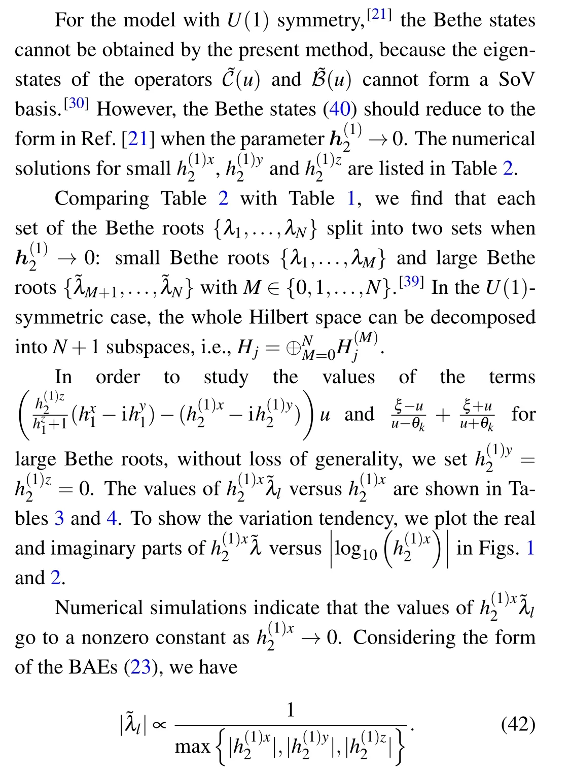
Table 2.Solutions of BAEs(23)for the case of N=3, j=1,{θk}={1.19,2.20,3.58},ξ =0.8i,ξ(1)=1.2,h=0.3,=0.5,=0.002i,=0.007i. The symbol n indicates the number of the eigenvalues,=Hj|ψ〉?|ψ〉,and is the corresponding energy. The energy calculated from Eq.(22)is the same as that from the exact diagonalization of the Gaudin Hamiltonian(1).

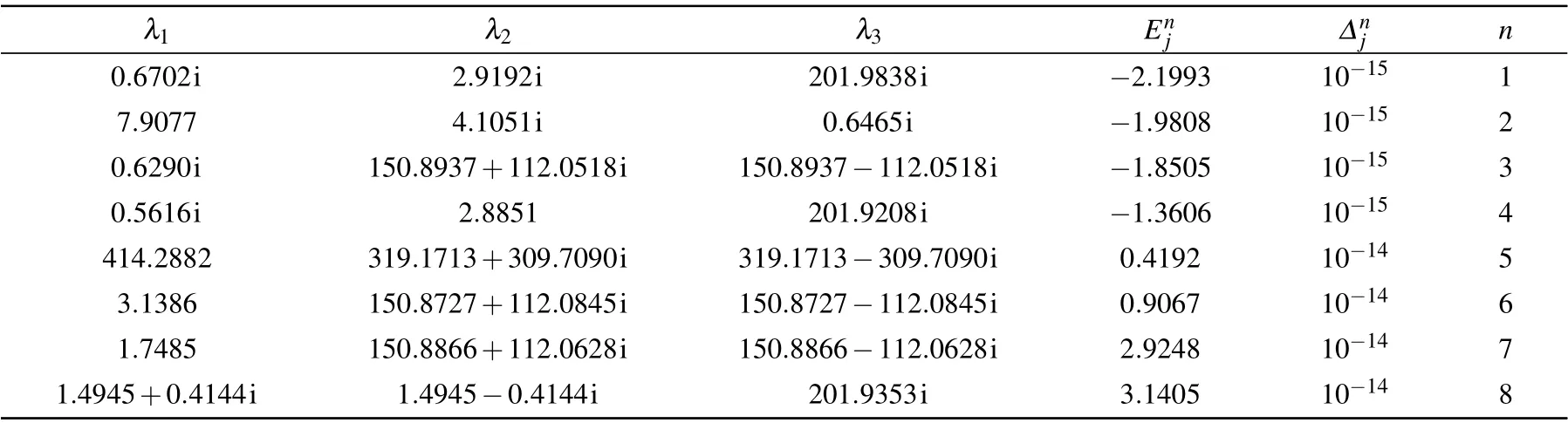
Table 2.Solutions of BAEs(23)for the case of N=3, j=1,{θk}={1.19,2.20,3.58},ξ =0.8i,ξ(1)=1.2,h=0.3,=0.5,=0.002i,=0.007i. The symbol n indicates the number of the eigenvalues,=Hj|ψ〉?|ψ〉,and is the corresponding energy. The energy calculated from Eq.(22)is the same as that from the exact diagonalization of the Gaudin Hamiltonian(1).

λ1 λ2 λ3 Enj ?nj n 0.6702i 2.9192i 201.9838i ?2.1993 10?15 1 7.9077 4.1051i 0.6465i ?1.9808 10?15 2 0.6290i 150.8937+112.0518i 150.8937?112.0518i ?1.8505 10?15 3 0.5616i 2.8851 201.9208i ?1.3606 10?15 4 414.2882 319.1713+309.7090i 319.1713?309.7090i 0.4192 10?14 5 3.1386 150.8727+112.0845i 150.8727?112.0845i 0.9067 10?14 6 1.7485 150.8866+112.0628i 150.8866?112.0628i 2.9248 10?14 7 1.4945+0.4144i 1.4945?0.4144i 201.9353i 3.1405 10?14 8

Table 3. Values of in solutions of BAEs(23)for the case of N=2, j=1,{θk}={1.19,2.20},ξ =0.8i,ξ(1)=1.2,=0,=0.7,h(1)y2 =0. The symbol n indicates the number of the eigenvalues.

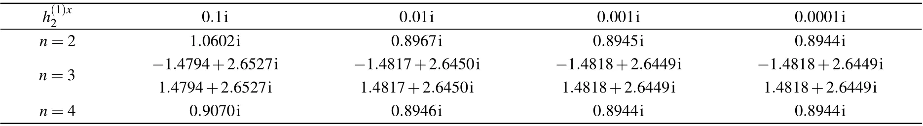
Table 3. Values of in solutions of BAEs(23)for the case of N=2, j=1,{θk}={1.19,2.20},ξ =0.8i,ξ(1)=1.2,=0,=0.7,h(1)y2 =0. The symbol n indicates the number of the eigenvalues.

h(1)x 2 0.1i 0.01i 0.001i 0.0001i n=2 1.0602i 0.8967i 0.8945i 0.8944i n=3 ?1.4794+2.6527i ?1.4817+2.6450i ?1.4818+2.6449i ?1.4818+2.6449i 1.4794+2.6527i 1.4817+2.6450i 1.4818+2.6449i 1.4818+2.6449i n=4 0.9070i 0.8946i 0.8944i 0.8944i

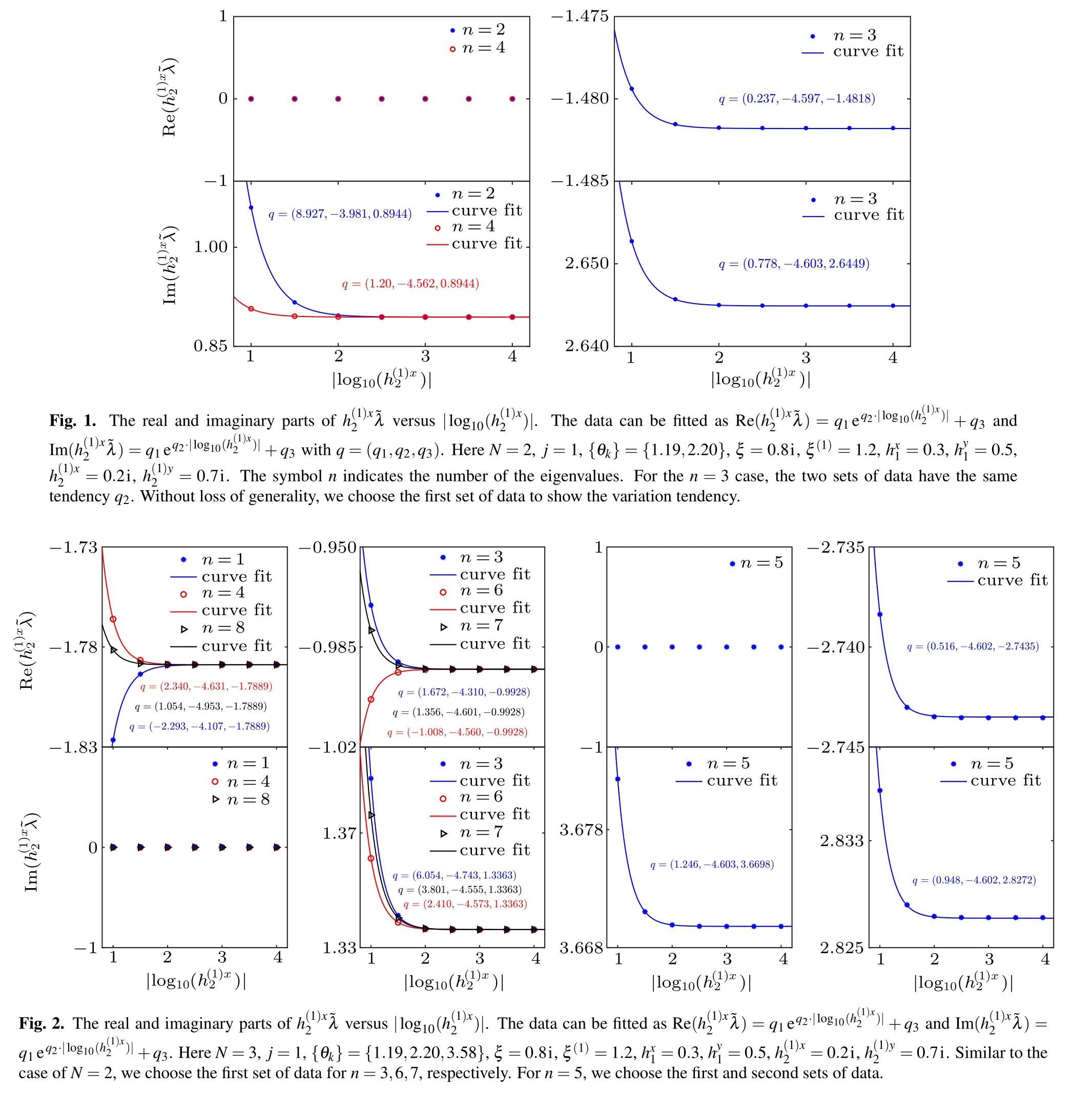
Table 4. Values of in solutions of BAEs (23) for the case of N =3, j=1, {θk}={1.19,2.20,3.58}, ξ =0.8i, ξ(1) =1.2, hx1 =0,=0.7,h(1)y2 =0. The symbol n indicates the number of the eigenvalues.

Table 4. Values of in solutions of BAEs (23) for the case of N =3, j=1, {θk}={1.19,2.20,3.58}, ξ =0.8i, ξ(1) =1.2, hx1 =0,=0.7,h(1)y2 =0. The symbol n indicates the number of the eigenvalues.

h(1)x 2 0.1i 0.01i 0.001i 0.0001i n=1 ?1.8265 ?1.7893 ?1.7889 ?1.7889 n=3 ?0.9704+1.3890i ?0.9925+1.3368i ?0.9928+1.3363i ?0.9928+1.3363i 0.9704+1.3890i 0.9925+1.3368i 0.9928+1.3363i 0.9928+1.3363i n=4 ?1.7661 ?1.7886 ?1.7889 ?1.7889 3.6823i 3.6699i 3.6698i 3.6698i n=5 ?2.7384+2.8368i ?2.7435+2.8273i ?2.7435+2.8272i ?2.7435+2.8272i 2.7384+2.8368i 2.7435+2.8273i 2.7435+2.8272i 2.7435+2.8272i n=6 ?1.0033+1.3612i ?0.9929+1.3365i ?0.9928+1.3363i ?0.9928+1.3363i 1.0033+1.3612i 0.9929+1.3365i 0.9928+1.3363i 0.9928+1.3363i n=7 ?0.9792+1.3762i ?0.9927+1.3367i ?0.9928+1.3363i ?0.9928+1.3363i 0.9792+1.3762i 0.9927+1.3367i 0.9928+1.3363i 0.9928+1.3363i n=8 ?1.7814 ?1.7888 ?1.7889 ?1.7889

This fact gives rise to

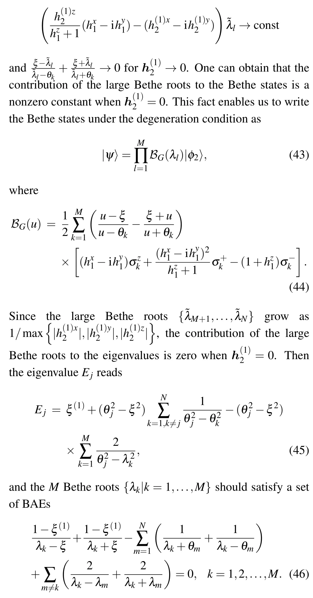
The numerical solutions of BAEs(46)and the corresponding eigenvalues(45)and Bethe states(43)of the Gaudin Hamiltonian(1)for N=3 are listed in Table 5.

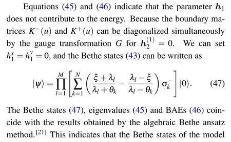
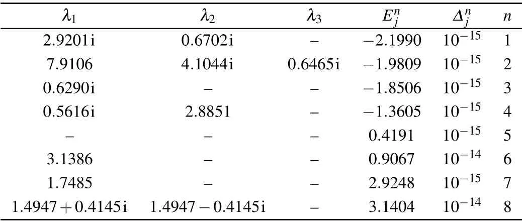
Table 5. Solutions of BAEs (46) for the case of N = 3, j = 1, {θk} ={1.19,2.20,3.58}, ξ =0.8i, ξ(1) =1.2, hx1 =0.4, hy1 =0.7. The symbol n indicates the number of the eigenvalues, ?nj =Hj|ψ〉?Enj|ψ〉, and Enj is the corresponding energy. The energy Enj calculated from Eq. (45) is the same as that from the exact diagonalization of the Gaudin Hamiltonian(1).

5. Conclusion

In summary, we have obtained the explicit closed-form expression of the Bethe states of the Gaudin model with DM and KSEA interactions. Taking the Gaudin model as a concrete example,we have studied the degeneration of the Bethe states(40). This method provide some insights into the degeneration of the Bethe states for other integral models without U(1)symmetry. In the near future,we will study the correlation functions and quantum dynamics of the Gaudin model(1)based on the results in this paper.

Appendix A:Proof of Eqs.(37)and(38)

In this appendix, we will construct the left Bethe state(37) and right Bethe state (38) of the inhomogeneous XXX Heisenberg spin chain.

A.1. Separation-of-variables(SoV)basis

With the help of the gauge transformation G, we introduce two local states of site n

It is easy to check that these states satisfy the orthogonal relationsj〈a|b〉k=δa,bδj,k, where a,b=1,2 and j,k=1,...,N.Using the above local states,we define

The SoV states can be constructed as[37]

It is easy to derive

A.2. Eigenstates of the inhomogeneous XXX Heisenberg spin chain

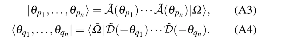
In Ref. [37], the key to construct the eigenstates 〈Ψ|of the transfer matrix t(u) is to calculate the scalar product 〈Ψ|θp1,...,θpn〉 with the SoV basis and the inhomogeneous T–Q relation (A16). For convenience, we denote〈Ψ|θp1,...,θpn〉as

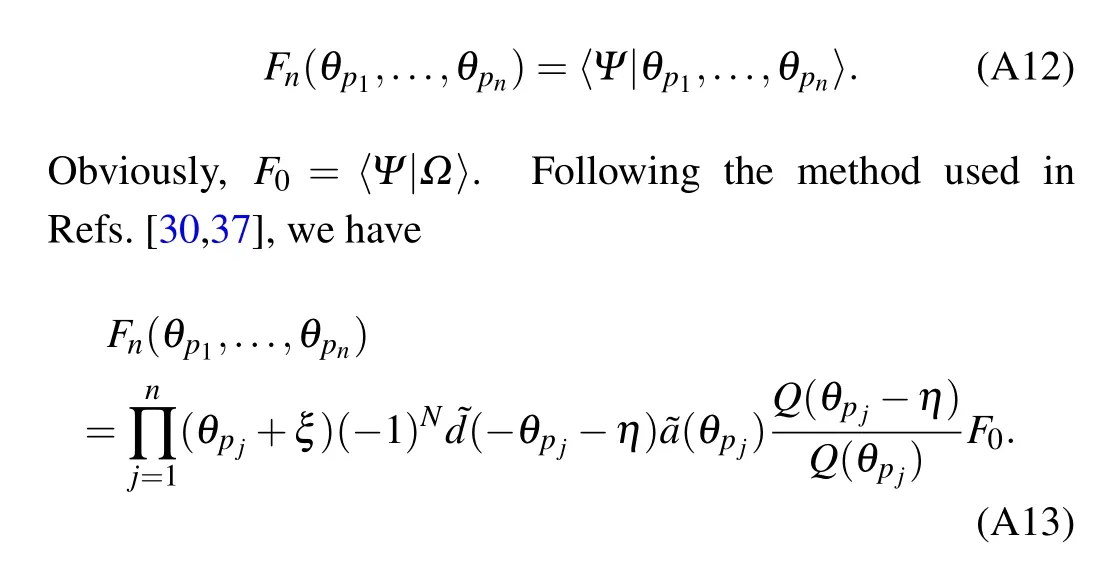
The eigenstates 〈Ψ| can be decomposed as a unique linear combination of the basis

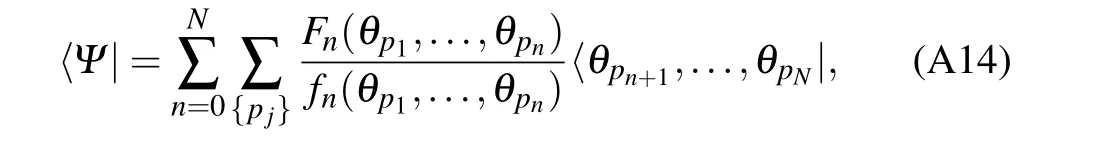
where p1＜···＜pnand pn+1＜···＜pN.

Based on the SoV basis and the inhomogeneous T–Q relation (A16), we construct the eigenstates of the transfer matrix t(u) (or the Hamiltonian HXXX= ?lnt(u)/?u|u=0).The benefit of this approach is that an reference states is not needed. Next,we construct the Bethe states of the inhomogeneous XXX Heisenberg spin chain using the SoV basis and the scalar product in Eq.(A13).

Acknowledgment

F.K.Wen would like to thank K.Hao for useful discussions. X.Zhang thanks the Alexander von Humboldt Foundation for financial support.