Furi–Martelli–Vignoli spectrum and Feng spectrum of nonlinear block operator matrices*

Xiao-Mei Dong(董小梅), De-Yu Wu(吳德玉),?, and Alatancang Chen(陳阿拉坦倉)

1School of Mathematical Sciences,Inner Mongolia University,Hohhot 010021,China

2Inner Mongolia Normal University,Hohhot 010021,China

Keywords: nonlinear operator,spectrum,block operator matrix

1. Introduction

Nonlinear operators are powerful tools for the study of nonlinear science. They are of great significance to the study of nonlinear functional analysis, differential equation and integral equation, and are widely applied in many fields such as mathematics, physics, biology and engineering.[1,2]In recent years,some topics of nonlinear operators have been studied in numerous articles.[3–6]In Ref. [7], the authors have discussed the solvability of nonlinear equations using some numerical characteristics of nonlinear operators. In Ref. [8],the authors have studied the uniqueness and existence of fixed points for a class of nonlinear operators,and applied their results to a class of integral equations. In view of the importance of nonlinear operators, spectra of nonlinear operators have been defined and studied by many researchers, and various definitions of spectra for nonlinear operators have been given.[9–18]One of them was introduced by Furi, Martelli and Vignoli in 1978.[15]This Furi–Martelli–Vignoli spectrum(FMV-spectrum,for short)of nonlinear operators shares some properties with the usual spectrum of bounded linear operators, such as it is always closed and sometimes even compact. In Ref. [16], another spectrum which is closely related to the FMV-spectrum was introduced by Feng in 1997. This Feng spectrum has similar topological properties as the FMVspectrum and contains all the eigenvalues. In particular,these two spectra have various applications to integeral equations,boundary value problems,and bifurcation theory.[11,15,16]

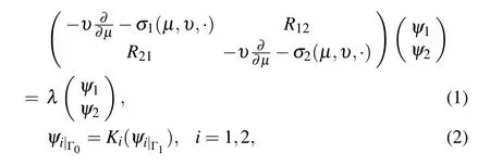
Many problems arising in mathematical physics and biology may be solved by nonlinear block operator matrices.For example, Ben Amar, Jeribi and Krichen[19]introduced and studied the existence of solutions for a coupled system of differential equations under abstract boundary conditions of Rotenberg’s model type,this last arises in growing cell populations. This problem is formulated by

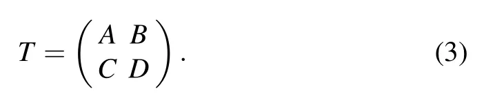
A lot of mathematicians have studied several kinds of linear operator matrices, and discussed the spectral properties and related subjects of these operator matrices.[20–28]Recently,the operator (3) with nonlinear entries has attracted increasing attention. Researchers have studied some fixed point theorems for the operator (3) on Banach spaces and Banach algebras,and applied these results to some systems of nonlinear equations.[19,29–34]However, few results have been reported on the spectral theory for nonlinear operator matrices.

This paper is devoted to studying the Furi–Martelli–Vignoli spectrum and Feng spectrum of continuous nonlinear block operator matrices. We mainly describe the relationship between the Furi–Martelli–Vignoli spectrum(compared to the Feng spectrum)of the whole operator matrix and that of its entries. In addition, the connection between the Furi–Martelli–Vignoli spectrum of the whole operator matrix and that of its Schur complement is presented by means of Schur decomposition.

Throughout this paper, let X and Y be infinite dimensional complex Banach spaces,and X×Y be a product space equipped with the norm

‖(x,y)‖=max{‖x‖,‖y‖}.

[F]A=inf{k:α(F(M))≤kα(M)},

[F]a=sup{k:α(F(M))≥kα(M)}.

We can write F ∈U(X,Y)if[F]A<∞. In the case of X =Y we can simply write U(X) instead of U(X,X). Observe that[F]A=0 if and only if F is compact,i.e.,the image F(M)of each bounded set M ?X is precompact in Y. The upper and lower quasinorms of F are defined as[11]

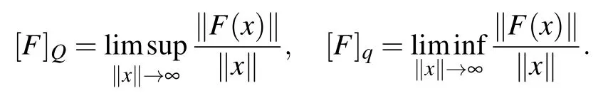
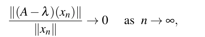
If[F]Q<∞,we call F quasibounded. Using Q(X,Y)denoting the set of all quasibounded operators from X to Y, as before,for X =Y we can simply write Q(X,X):=Q(X). Moreover,[F]q>0 implies that F is coercive,i.e. ,

We also consider

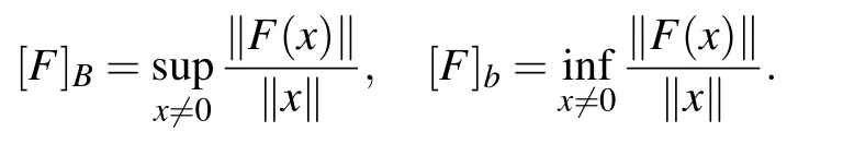
In the case of[F]B<∞,we can write F ∈B(X,Y)and call the operator F linearly bounded, and B(X,X):=B(X)as before.From the definition and our general assumption F(0)=0 it follows that

[F]b≤[F]q≤[F]Q≤[F]B.

2. The Furi–Martelli–Vignoli spectrum of nonlinear block operator matrices

In this section, we first introduce some definitions and some auxiliary lemmas which will be used later.

Definition 2.1[36]A continuous operator F :X →Y can be stably solvable if for any continuous compact operator G : X →Y with [G]Q=0, the equation F(x)=G(x) has a solution x ∈X.

Remark 2.1Each stably solvable operator is surjective,but in general the converse is not true. For linear operators,however,surjectivity is equivalent to stable solvability.

Definition 2.2[15]A continuous operator F :X →X is FMV-regular if F is stably solvable, [F]a>0 and [F]q>0.The set

ρFMV(F)={λ ∈C:F ?λI is FMV-regular}

is called the FMV-resolvent set of F,and its complement σFMV(F)=C?ρFMV(F)

is called the FMV-spectrum of F. Also,the sets

σδ(F)={λ ∈C:F ?λI is not stably solvabl},

σπ(F)=σq(F)∪σa(F)

are called the defect spectrum and approximate point spectrum of F,respectively,where

σq(F)={λ ∈C:[F ?λI]q=0},

σa(F)={λ ∈C:[F ?λI]a=0}.

Obviously

σFMV(F)=σδ(F)∪σπ(F)=σδ(F)∪σa(F)∪σq(F).

Remark 2.2In the case of a bounded linear operator F,σπ(F) is the approximate point spectrum of F, σδ(F) is the defect spectrum of F, and σFMV(F) is the usual spectrum of F.

Lemma 2.1[15]Let X and Y be Banach spaces and M ?X, N ?Y be bounded subsets. Consider X×Y with the norm

‖(x,y)‖=max{‖x‖,‖y‖}.

Then

α(M×N)=max{α(M),α(N)}.

Lemma 2.2[15]Let X and Y be Banach spaces, F,G ∈C(X,Y). Then

(1)[F]a[G]a≤[FG]a≤[F]A[G]a;

(2)[F]q[G]q≤[FG]q≤[F]Q[G]q;

(3)[F]a?[G]A≤[F+G]a≤[F]a+[G]A;

(4)[F]q?[G]Q≤[F+G]q≤[F]q+[G]Q.

Lemma 2.5[11]Let X be a Banach space,F ∈C(X).Suppose that F satisfies [F]A<1 and [F]Q<1. Then I ?F is surjective;in particular,F has a fixed point in X.

Next, we describe the relationship between the FMVspectrum of the whole operator matrix and its entries.

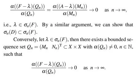
Set Qn=(Mn0)T?X×X,n ∈N. Clearly,α(Qn)=α(Mn)and α((F ?λ)(Qn))=α((A?λ)(Mn)). Thus

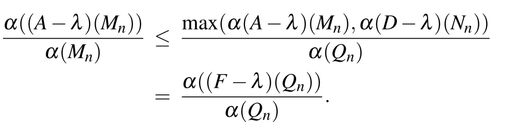
From Lemma 2.1,we know that α(Qn)=max{α(Mn),α(Nn)}.Without loss of generality we may assume that α(Qn) =α(Mn)for infinitely many indices n,then

Thus

i.e.,λ ∈σa(A). The proof for λ ∈σa(D)is similar. Therefore,σa(F)=σa(A)∪σa(D).

(ii)Let λ ∈σq(A),then there exists a sequence{xn}∞n=1?X with‖xn‖→∞,such that

Set zn=(xn0)T∈X×X,then‖zn‖→∞,and

i.e.,λ ∈σq(F). Similarly,we can show that σq(D)?σq(F).

Without loss of generality we may assume that ‖xn‖≥‖yn‖for infinitely many indices n,then‖xn‖→∞,and

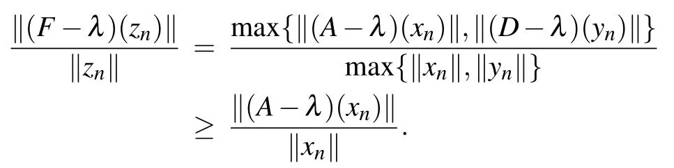
Thus

i.e., λ ∈σq(A). The proof for λ ∈σq(D) is similar. Consequently,σq(F)=σq(A)∪σq(D).

(iii) To show that σδ(F)?σδ(A)∪σδ(D), it suffices to show that if F is stably solvable then so are A and B. If F is stably solvable,let H1:X →X and H2:X →X are continuous compact operators with [H1]Q=0 and [H2]Q=0. Define an operator H:X×X →X×X by

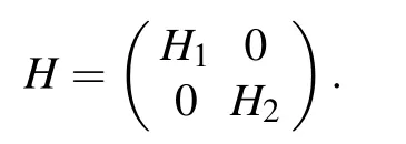
Clearly,H is a compact operator and[H]Q=0.Then

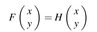
has a solution(x y)T∈X×X,i.e.,

A(x)=H1(x) and D(y)=H2(y),

which implies that both of A and D are stably solvable.

(iv)From(i)–(iii),it is clear that σFMV(A)∪σFMV(D)?σFMV(F), now we prove that σFMV(F) ?σFMV(A) ∪σFMV(D)∪σ+(A)∪σ+(D). Let λ /∈σFMV(A)∪σFMV(D)∪σ+(A)∪σ+(D),then[A?λ]a>0,[A?λ]q>0,[D?λ]a>0,[D ?λ]q>0 and A ?λ, D ?λ are homeomorphisms on X,therefore [F ?λ]a>0, [F ?λ]q>0 and F ?λ is a homeomorphism on X×X. Let H :X×X →X×X is a continuous compact operator with[H]Q=0,then

[(F ?λ)?1H]A≤[(F ?λ)?1]A[H]A=0

and

[(F ?λ)?1H]Q≤[(F ?λ)?1]Q[H]Q=0.

From Lemma 2.5,it follows that(F ?λ)?1H has a fixed point in X×X, and hence F ?λ is stably solvable. This together with[F ?λ]a>0 and[F ?λ]q>0 implies that λ /∈σFMV(F).

σFMV(A)∪σFMV(D)=σFMV(F)

if and only if

σ+(A)∪σ+(D)?σFMV(F).

In particular, if σ+(A) ∪σ+(D) = ?, then σFMV(A) ∪σFMV(D)=σFMV(F).

Remark 2.3 For bounded linear diagonal operator matrices,obviously,σ+(A)∪σ+(D)?σFMV(F).

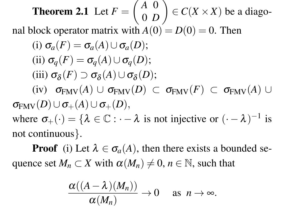
(i)σa(A)?σa(F)?σa(A)∪σa(D);

(ii)σq(A)?σq(F)?σq(A)∪σq(D).

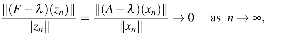
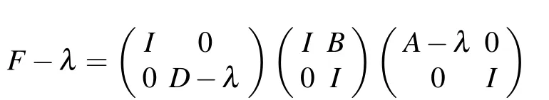
Proof (i) It is easy to see that σa(A)?σa(F), and so we only need to prove that σa(F) ?σa(A)∪σa(D). Let λ ∈σa(F), then [F ?λ]a= 0. Evidently, the factorization formula

(ii)The proof is analogous to(i),and its proof is omitted here.

It is easy to get the following corollary.

σπ(A)?σπ(F)?σπ(A)∪σπ(D).

According to Corollary 2.2,we can estimate the distribution range of set (σπ(A)∪σπ(D))?σπ(F), see the following theorem.

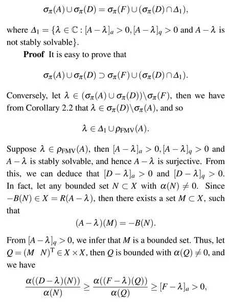
which implies that[D?λ]a>0. We can obtain[D?λ]q>0 by a similar method. This contradicts λ ∈σπ(D). Then λ ∈?1,therefore

(σπ(A)∪σπ(D))?σπ(F)?σπ(D)∩?1.

Remark 2.5 In Theorem 2.3,if further A ∈L(X),then

Since λ /∈σπ(F),then

[M]a=[(F ?λ)V]a≥[F ?λ]a[V]a>0

and

[M]q=[(F ?λ)V]q≥[F ?λ]q[V]q>0,

therefore[D?λ]a>0 and[D?λ]q>0,so the desired result follows from the proof of Theorem 2.3.

According to Theorem 2.3 and Remark 2.5,we immediately have the following corollaries.

σπ(A)∪σπ(D)=σπ(F)

if and only if

σπ(D)∩?1?σπ(F).

In particular, if σπ(D)∩?1= ?, then σπ(A)∪σπ(D) =σπ(F).

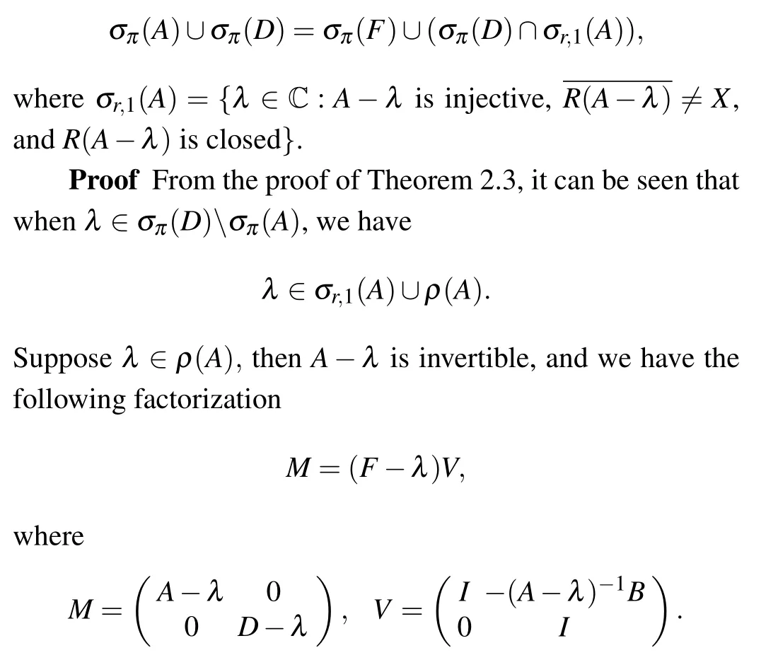
A ∈L(X)and B ∈U(X)∩Q(X),then

σπ(A)∪σπ(D)=σπ(F)

if and only if

σπ(D)∩σr,1(A)?σπ(F).

In particular, if σπ(D)∩σr,1(A)=?, then σπ(A)∪σπ(D)=σπ(F).

Remark 2.6For linear (not necessary bounded) upper triangular operator matrices,Theorem 2.3,Corollaries 2.3 and 2.4 are also valid, where ?1=σr,1(A). Readers can see Refs.[24].

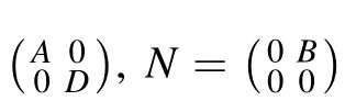
In Ref. [21], it was shown that if N and M are bounded linear operators, and satisfy N2= 0 and either NM = 0 or MN=0,then

(i)σa(F)?{0}=(σa(A)∪σa(D))?{0};

(ii)σq(F)?{0}=(σq(A)∪σq(D))?{0};

(iii)σδ(F)?σδ(A)∪σδ(D);

(iv)σFMV(F)?σFMV(A)∪σFMV(D).

Let us give an example to show that the statement(ii)of Corollary 2.5,in general,is not true when the spectral point is zero.

Example 2.1Let X be an infinite dimensional complex Banach space with the maximum norm, e=(1,0,0,...)∈X,and

A1(x)=A2(x)=D1(x)=‖x‖e, Sr(x)=(0,x1,x2,···)

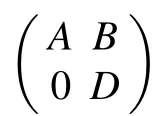
for x=(x1,x2,...)∈X. Consider the block operator matrix

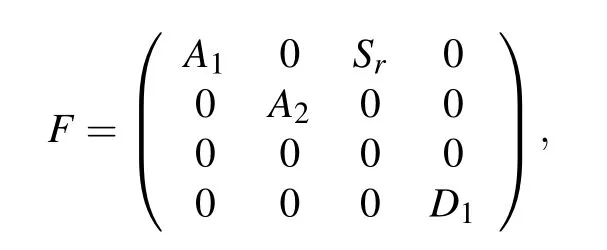
where

Theorem 2.5Let M,N ∈C(X).

(i)If[N]A=0,then σa(M+N)=σa(M).

(ii)If[N]Q=0,then σq(M+N)=σq(M).

(iii)If[N]A=0 and[N]Q=0,then σδ(M+N)=σδ(M).

(iv) If [N]A= 0 and [N]Q= 0, then σFMV(M+N) =σFMV(M).

ProofThe proof is trivial,and its proof is omitted here.

(i)If[B]A=0,then σa(F)=σa(A)∪σa(D).

(ii)If[B]A=0 and[B]Q=0,then σq(F)=σq(A)∪σq(D).

(iii) If [B]Q= 0 and [B]A= 0, then σδ(F) ?σδ(A)∪σδ(D).

(iv)If[B]Q=0 and[B]A=0,then σFMV(F)?σFMV(A)∪σFMV(D).

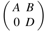
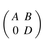
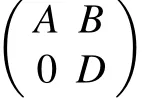
In the theory of bounded and unbounded linear block operator matrices, Schur complements are powerful tools to study the spectrum and various spectral properties,see the series of papers.[37–39]Given a linear block operator matrix

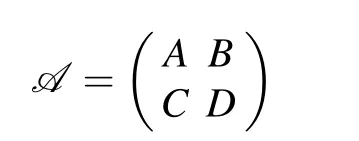
defined on the product Banach space X1×X2of two Banach spaces X1,X2. Then

and

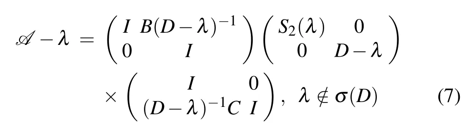
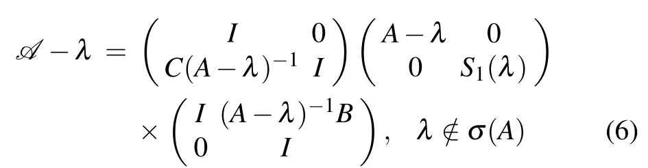
are called the Frobenius–Schur factorization,where

S1(λ)=D?λ ?C(A?λ)?1B, λ /∈σ(A)

and

S2(λ)=A?λ ?B(D?λ)?1C, λ /∈σ(D)are called the Schur complements of A.

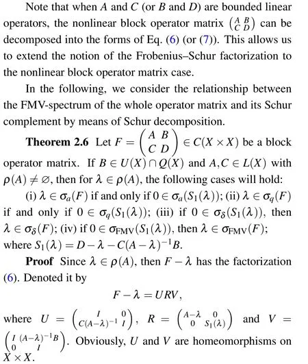
(i) Let λ ∈σa(F), then [F ?λ]a=0. Since [U]a>0,[V]a>0 and

[F ?λ]a=[URV]a≥[U]a[R]a[V]a,

it follows that [R]a= 0, and hence [S1(λ)]a= 0, i.e., 0 ∈σa(S1(λ)).Conversely,let 0 ∈σa(S1(λ)),then[R]a=0.Since[U?1]a>0,[V?1]a>0 and

[R]a=[U?1(F ?λ)V?1]a≥[U?1]a[F ?λ]a[V?1]a,

then we have that[F ?λ]a=0,i.e.,λ ∈σa(F).

(ii)The proof is similar to(i).

(iii)Since U,V,U?1and V?1are all quasibounded.Then,by Lemma 2.3 and Lemma 2.4,we obtain that F ?λ is stably solvable if and only if R is stably solvable. Thus, if F ?λ is stably solvable,then applying Theorem 2.1,we can infer that S1(λ)is stably solvable. So we complete the proof.

(iv) It follows immediately from (i)–(iii) and the definition of the FMV-spectrum.

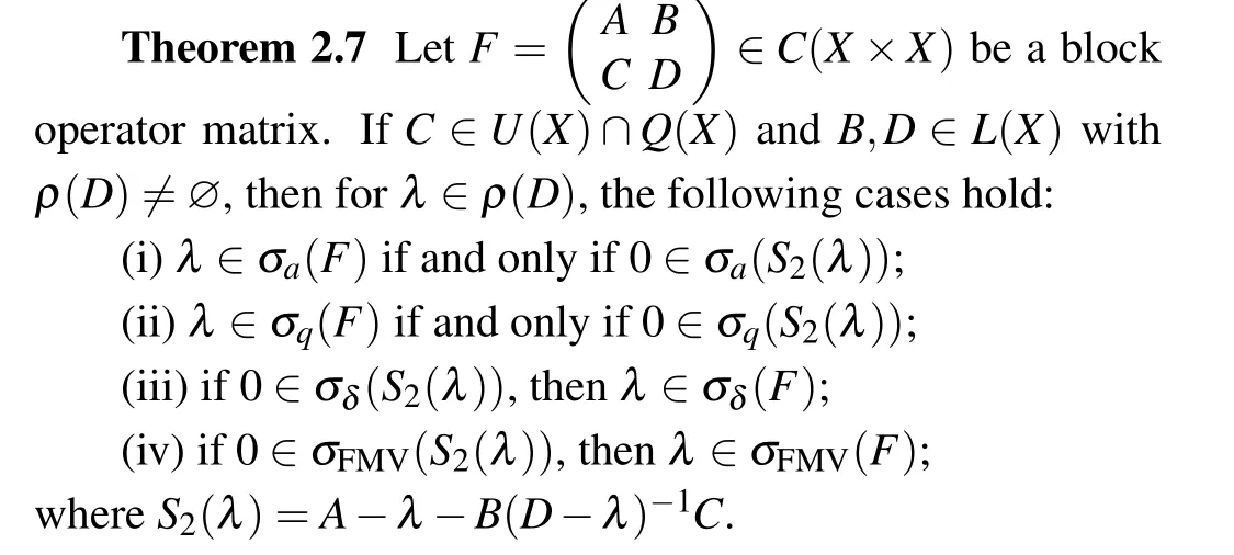
ProofThe proof is analogous to that of Theorem 2.6,we only need to note that when λ ∈ρ(D), F ?λ has the factorization(7).

From the proofs of Theorems 2.6 and 2.7,we find the following theorem.

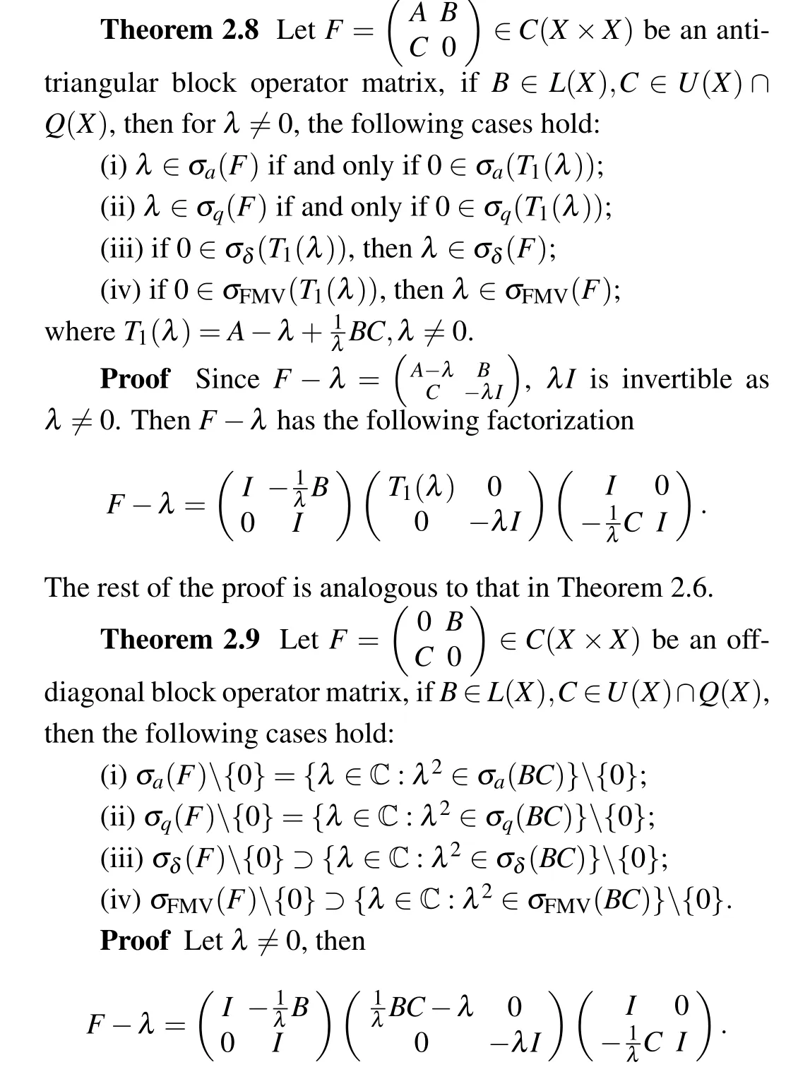
Similar to the proof of Theorem 2.6,we have

Thus,we immediately have the assertions(i)–(iii)and(iv)hold.

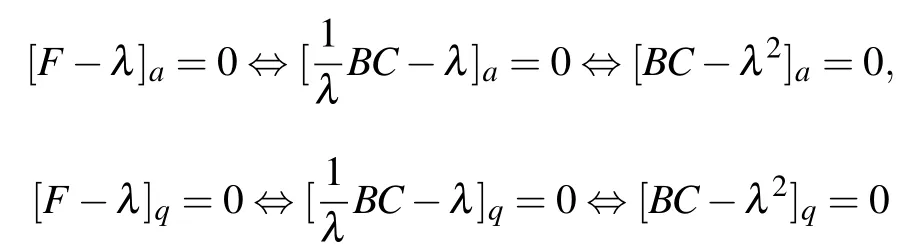
(i)σa(F)?{0}={λ ∈C:λ2∈σa(CB)}?{0};

(ii)σq(F)?{0}={λ ∈C:λ2∈σq(CB)}?{0};

(iii)σδ(F)?{0}?{λ ∈C:λ2∈σδ(CB)}?{0};

(iv)σFMV(F)?{0}?{λ ∈C:λ2∈σFMV(CB)}?{0}.

Finally,we end this section with an example to illustrate the previous results.

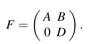
Example 2.2Let X be an infinite dimensional complex Banach space,e ∈X with‖e‖=1,and

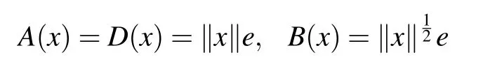
for x ∈X. Consider the block operator matrix

Then by Theorem 2.3, we have (σπ(A)∪σπ(D))?σπ(F) =σπ(D)∩?1.Furthermore,by Corollary 2.3,we have σπ(F)=σπ(A)∪σπ(D),where ?1={λ ∈C:[A?λ]a>0,[A?λ]q>0 and A?λ is not stably solvable}.

On the other hand, since A, B and D are compact operators,then σa(A)=σa(D)=σa(F)=0.Moreover,by calculation,we have[11]

σq(A)=σq(D)=?D, σδ(A)=σδ(D)=D,

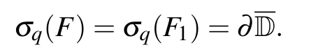
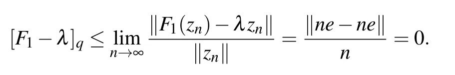
i.e.

λ ∈σq(F1).

In summary,

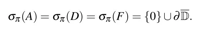
?1={λ ∈C:[A ?λ]a>0,[A ?λ]q>0 and A ?λ is not stably solvable}=D?{0}.

Thus

σπ(A)∪σπ(D)?σπ(F)=?, σπ(D)∩?1=?.

Therefore

(σπ(A)∪σπ(D))?σπ(F)=σπ(D)∩?1.

Furthermore

σπ(F)=σπ(A)∪σπ(D).

This shows that Theorem 2.3 and Corollary 2.3 are valid.

3. The Feng spectrum of nonlinear block operator matrices

Let X and Y be infinite dimensional complex Banach spaces and denote by DBC(X) the family of all open,bounded,connected subsets ? of X with 0 ∈?.Let F:X →Y be a continuous nonlinear operator.

F(x)=G(x)

and

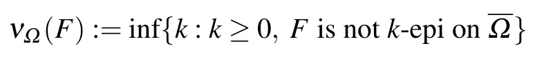
Definition 3.2[11]A continuous operator F :X →X is F-regular if[F]a>0,[F]b>0 and ν(F)>0. The set

ρF(F)={λ ∈C:F ?λI is F-regular}

is called the Feng-resolvent set of F,and its complement

σF(F)=C?ρF(F)

is called the Feng-spectrum of F.

Obviously

σF(F)=σa(F)∪σb(F)∪σν(F),

where

σa(F)={λ ∈C:[F ?λI]a=0},

σb(F)={λ ∈C:[F ?λI]b=0},

σv(F)={λ ∈C:ν(F ?λI)=0}.

Remark 3.1Every F-regular operator F :X →X is surjective. Furthermore, L ∈L(X) is F-regular operator if and only if L is an isomorphism.

Definition 3.3[11]A continuous operator F :X →Y is called k-stably solvable (k ≥0) if for any continuous operator G : X →Y with [G]A≤k and [G]Q≤k, the equation F(x)=G(x)has a solution x ∈X.

For F ∈C(X,Y),we can call the number

μ(F):=inf{k:k ≥0, F is notk-stably solvable}

the measure of stable solvability of F. Also, we can say that a continuous operator F :X →Y is strictly stably solvable ifμ(F)>0,i.e.,F is k-stably solvable for some positive k.

The next lemma provides a connection between FMVregular operator and strictly stably solvable operators.

Lemma 3.1[11]Every FMV-regular operator F :X →Y is strictly stably solvable. More precisely,the estimate

μ(F)≥min{[F]q, [F]a}

holds.

The next lemma connects the measure of solvability and the measure of stable solvability of F.

Lemma 3.2[11]For any continuous operator F :X →Y,we have the estimate

μ(F)≤ν(F).

In the following,we describe the relationship between the Feng-spectrum of the whole operator matrix and its entries.

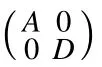
Theorem 3.1Let F ∈C(X×X) be the diagonal block operator matrix as in Theorem 2.1. Then

σF(F)?σF(A)∪σF(D)∪σ+(A)∪σ+(D),

where σ+(·)={λ ∈C:·?λ is not injective or (·?λ)?1is not continuous}.

ProofLet λ /∈σF(A)∪σF(D)∪σ+(A)∪σ+(D)),then,by the proof of Theorem 2.1, we know that F ?λ is FMVregular operator, therefore μ(F ?λ)>0 by Lemma 3.1, and we have from Lemma 3.2 that λ /∈σF(F).

Let σ?(F)=σa(F)∪σb(F), we have the following results which are similar to Theorem 2.3 and Corollaries 2.2–2.4, and can be proved in a similar way, so their proofs are omitted here.

Theorem 3.2Let F ∈C(X×X)be the upper triangular block operator matrix as in Corollary 2.2.If B ∈U(X)∩B(X),then

σ?(A)?σ?(F)?σ?(A)∪σ?(D).

Theorem 3.3Let F ∈C(X×X)be the upper triangular block operator matrix as in Theorem 2.3. If B ∈U(X)∩B(X)and A(0)=0,then

σ?(A)∪σ?(D)=σ?(F)∪(σ?(D)∩?2),

where ?2={λ ∈C:[A?λ]a>0,[A?λ]b>0 and ν(A?λ)=0}.

Corollary 3.1Let F ∈C(X×X)be the upper triangular block operator matrix as in Theorem 2.3. If B ∈U(X)∩B(X)and A(0)=0,then

σ?(A)∪σ?(D)=σ?(F)

if and only if

σ?(D)∩?2?σ?(F).

In particular, if σ?(D)∩?2= ?, then σ?(A)∪σ?(D) =σ?(F).

Theorem 3.4Let F ∈C(X×X) be the upper triangular block operator matrix as in Theorem 2.3. If A ∈L(X)and B ∈U(X)∩B(X),then

σ?(A)∪σ?(D)=σ?(F)∪(σ?(D)∩σr,1(A)),

where σr,1(A)is defined as in Remark 2.5.

Corollary 3.2Let F ∈C(X×X) be the upper triangular block operator matrix as in Theorem 2.3. If A ∈L(X)and B ∈U(X)∩B(X),then

σ?(A)∪σ?(D)=σ?(F)

if and only if

σ?(D)∩σr,1(A)?σ?(F)).

In particular, if σ?(D)∩σr,1(A)=?, then σ?(A)∪σ?(D)=σ?(F).

4. Conclusions

Block operator matrix plays a significant role in system theory, quantum mechanics, hydrodynamics and magnetohydro-dynamics. In this paper, we obtain some connections between the FMV-spectrum (compared to the Feng spectrum)of the diagonal as well as upper triangular nonlinear operator matrix and that of their diagonal entries. In addition,the relationship between the FMV-spectrum of the whole 2×2 nonlinear operator matrix and that of its Schur complement is presented by means of Schur decomposition. This provides a theoretical basis for solving systems of nonlinear equations in mathematical physics.