INITIAL BOUNDARY VALUE PROBLEM FOR THE 3D MAGNETIC-CURVATURE-DRIVEN RAYLEIGH-TAYLOR MODEL?
2020-06-04 08:50:44
School of Mathematics and Information Science,Guangzhou University,Guangzhou 510006,China
E-mail:puxueke@gmail.com
Boling GUO
Institute of Applied Physics and Computational Mathematics,P.O.Box 8009,Beijing 100088,China
E-mail:gbl@iapcm.ac.cn
Abstract This article studies the initial-boundary value problem for a three dimensional magnetic-curvature-driven Rayleigh-Taylor model.We first obtain the global existence of weak solutions for the full model equation by employing the Galerkin’s approximation method.Secondly,for a slightly simplified model,we show the existence and uniqueness of global strong solutions via the Banach’s fixed point theorem and vanishing viscosity method.
Key words Magnetic-curvature-driven Rayleigh-Taylor model;weak solutions;strong solutions;Banach fixed point theorem;vanishing viscosity method
1 Introduction
The magnetic-curvature-driven Rayleigh-Taylor model is a useful paradigm for the study of the long wave length nonlinear shear flow patterns such as the zonal flows and streamer structures.The PDE model reads
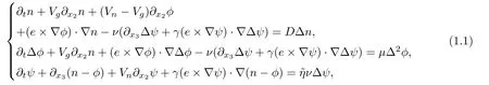
where n is the plasma density, φ is the scalar electric field potential,and ψ is the parallel component of the magnetic vector potential for electromagnetic perturbations.Here,e=(0,0,1)is the unit vector in the x3-direction,Vnand Vgare,respectively,the diamagnetic drift speed and the gravitational drift arising through the magnetic curvature terms,μand D are the dynamical viscosity and the diffusion coefficient,ν1/2is the normalized Alfvén velocity,andand γ are dimensionless parameters.Here,represents the resistivity coefficient appearing in the Ohm’s law and in the following,we will denote.This model plays an important role in determining the turbulent transport of matter and heat across field lines in magnetically confined plasma devices such as tokamaks,stellarators,etc.([1]).
When the electromagnetic perturbations ψ is independent of x3,the first two equations are not influenced in any way by ψ.Although the evolution of ψ is driven by n and φ,but ψ is unable to react back on n and φ.Under this limit,after several mathematical treatments,the model equation(1.1)is simplified into the following 2D model equation
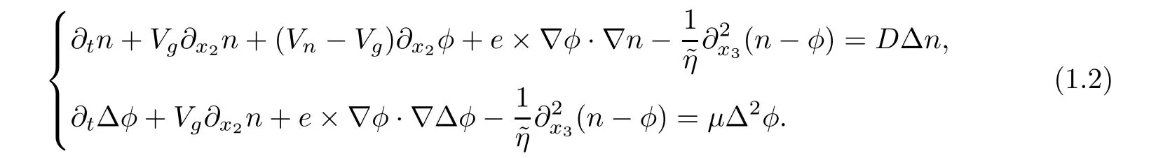
This model was proposed in 1983 by Hasegawa and Wakatani for a two- fluid model describing the resistive drift wave turbulence in Tokamak(see[5,6]).Recently,Kondo and Tani proved the global(resp.local)existence and uniqueness of strong solutions for the initial and boundary problems for(1.2)with Vn=Vg=0 when D>0(resp.D=0)(see[11]).Further simplifications for this equation can reduce this equation into the Hasegawa-Mima equation proposed in 1977 by Hasegawa and Mima(see[3,4])for one fluid model in a homogeneous strong magnetic field and an inhomegeneous plasma equilibrium density.See[2,12,13]for its well-posedness and long-time dynamical behaviors.Comparing(1.1)with the 2D model,we see that the 3D model(1.1)has both linear and nonlinear coupling to the magnetic perturbation and is more relativistic.
The mathematical study for(1.1)is not easy because it is highly nonlinear in ψ and no general mathematical theory can be applied.Hence,we turn to consider the following simplified model when the nonlinear coupling to the magnetic perturbation is very weak(that is,letting γ=0 in(1.1))
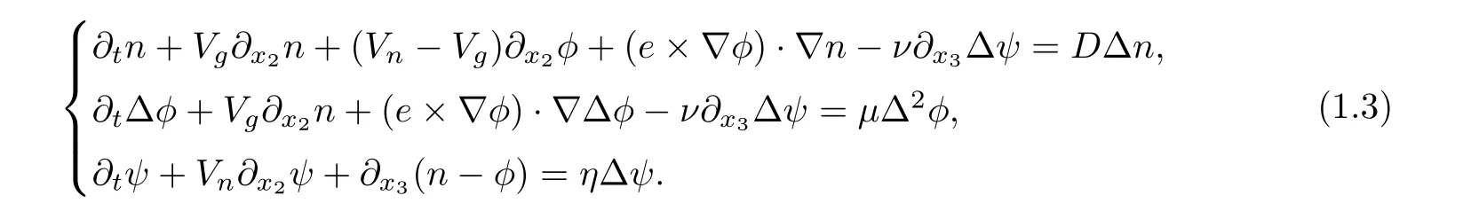
This model equation keeps all the important features in physics when the nonlinear coupling is weak,but is simplified greatly mathematically.
In this article,we study the global existence of weak solution for(1.1)and global existence of strong solutions for(1.3)for D≥0 under the following initial and boundary conditions
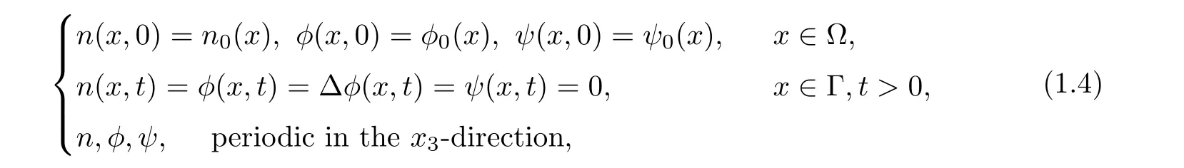
where ? = ω ×(?L,L)is a three dimensional torus,and R and L are positive real numbers.We note that only local existence of strong solutions for(1.2)is obtained when D=0 in[11].
In the following,we state the main results in this article.First,we give the definition of weak solutions for(1.1).
Definition 1.1Let T>0 be arbitrary.(n,φ,ψ)is called a weak solution for(1.1)in[0,T]under initial boundary conditions(1.4),provided that
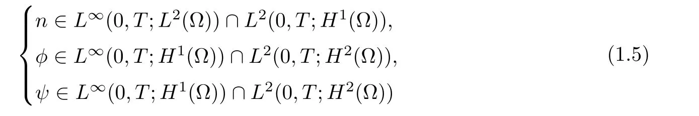
and satisfies system(1.1)in the weak sense
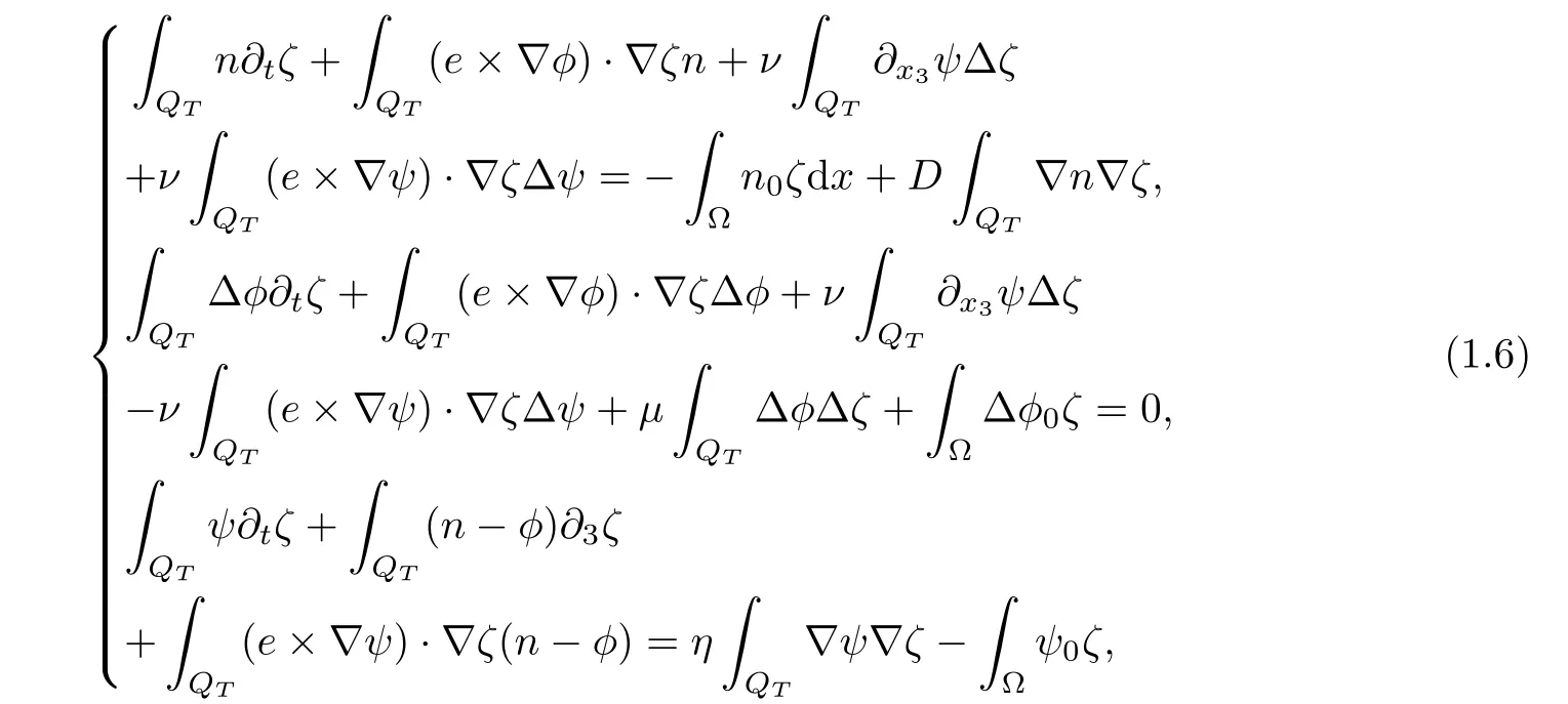
The global existence of weak solutions can be obtained by the standard Galerkin approximation method and the following theorem will be proved.
Theorem 1.2Let D>0 and(n0,φ0,ψ0)∈ L2(?)×H1(?)×H1(?).Then for any T>0,there exists a weak solution(n,φ,ψ)for(1.1)in the sense of Definition 1.1.
Remark 1.3Similar result on existence of global weak solutions still holds when D=0.In this case,we only have n ∈ L∞(0,T;L2(?)).But this will not introduce any difficulties in showing the global existence of weak solutions in the sense of Definition 1.1,as can be seen through the proof of Theorem 1.2 in Section 2.
Next,we show the local and global existence for strong solution for(1.3)under the initialboundary conditions(1.4).
Theorem 1.4Let Vn=Vg=0,1/2
the initial boundary value problem(1.3)and(1.4)has a unique solutionfor any T>0.
On the other hand,letting D=0,we can prove the following
Theorem 1.5Assume thatsatisfies the compatibility condition in(1.7),then there exists a unique solutionto the initial boundary value problem(1.3)and(1.4)with D=0 for any T>0.
In what follows,we review the notations used throughout this article.Let ? be a domain in Rmfor m positive integers,then we useand(·,·)to denote the L2(?)norm and L2-inner product,respectively. Sometimes,we simply useto denote the L2(?)norm without introducing any confusions.For l∈ R,l≥ 0,we defineto be the space of functions u(x),x ∈ ? such thatis defined aswhen l is a nonnegative integer and when l is not an integer,we defineHere,[l]is the integer part of l,with α =(α1,···,αm)and=α1+···+αm.Let QT= ?×(0,T),and the anisotropic Sobolev-Slobodetskii spaceis defined asequipped with the norm

We will also use the following notations. We will useto denote the space of functions u such thatInterpolation between these spaces can be found in[9].For notational simplicity,we denote,i=1,2,3,and
This article is organized as follows.In the next section,we prove Theorem 1.2 by Galerkin approximation method.In Section 3,we prove Theorem 1.4 by Banach’s fixed point theorem combined with some global a priori estimates.In Section 4,we prove Theorem 1.5 by providing a priori estimates independent of D.In the following three sections,let Vn=Vg=0 only for mathematical simplification.Whenthe results can be proved by parallel reasoning without any difficulties.
2 Global Strong Solutions
We only provide the formal estimates in the following lemma.
Lemma 2.1Let D≥0,then for any T>0,there exists some constant CTdepending only on ν,μ,η and T such that
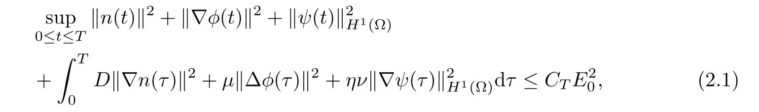
ProofMultiply the first equation in(1.1)with n and then integrate over ? to obtain via integration by parts

Similarly,from the second equation in(1.1),we obtain

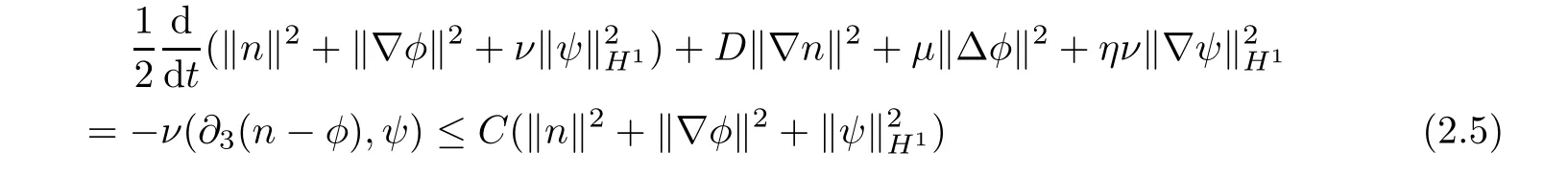
Adding(2.2),(2.3)and(2.4)multiplied by ν,and then integrating by parts yields
Lemma 2.2Under the conditions of Lemma 2.1,there exists a constant K such that

where H?3(?)is the dual of
ProofThis can be proved by directly using system(1.1)and the dual method.The estimates in Lemmas 2.1 and 2.2 are formal,but can be made rigorous for an appropriate sequence of approximations{nN,φN,ψN},for example,the Galerkin truncations.These estimates show that the approximate solutions(nN,φN,ψN)are uniformly(in N)bounded in V=(L∞(0,T;L2)∩L2(0,T;H1))×(L∞(0,T;H1)∩L2(0,T;H2))×(L∞(0,T;H1)∩L2(0,T;H2)).Therefore,there exists(n,φ,ψ) ∈ V such that(nN,φN,ψN) → (n,φ,ψ)in V up to a subsequence as N→∞.On the other hand,Lemma 2.2 together with the compactness theorem in[10,Theorem 5.1]shows that(nN,φN,ψN)is compact in intermediate spaces L2(0,T;Hs)×L2(0,T;H2+s)×L2(0,T;H2+s)for s<0.
For each N ∈ N,(1.6)holds for any test functionwith ζ(x,t)|Γ=0,ζ(T)=0.To show that(nN,φN,ψN)converges to a weak solution as N → ∞,it suffices to show the convergence of the nonlinear terms.We take the following term as an example.We need to show that

However,by the compactness of the approximate sequence,we have
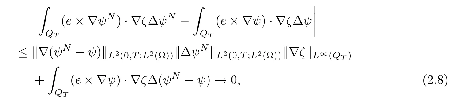
where the last term converges to zero because ψN→ ψ weakly in L2(0,T;H2(?))and strongly in L2(0,T;H1(?)).
We also note that for D=0,the above argument still holds with minor modifications.Therefore,the proof of Theorem 1.2 is complete.
3 Global Strong Solutions
In this section,we show the global-in-time existence of solutions for the initial-boundary value problem(1.3)and(1.4)with D≥0.This is divided into two parts.First,we show the local-in-time existence of solutions by iteration and Banach fixed point theorem.Then,we make some a priori estimates,which together with the local existence will yield the global existence of strong solutions.
3.1 Local existence
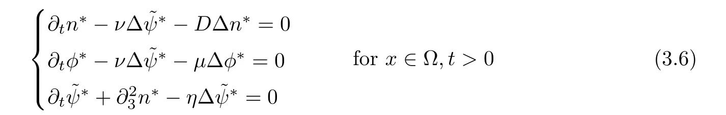
To study the local-in-time existence and uniqueness,we first setto transform the third equation of(1.3)into(note we have set Vn=Vg=0)

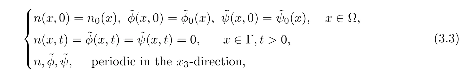
This leads us to consider the linear parabolic equation for(n,=?φ,)
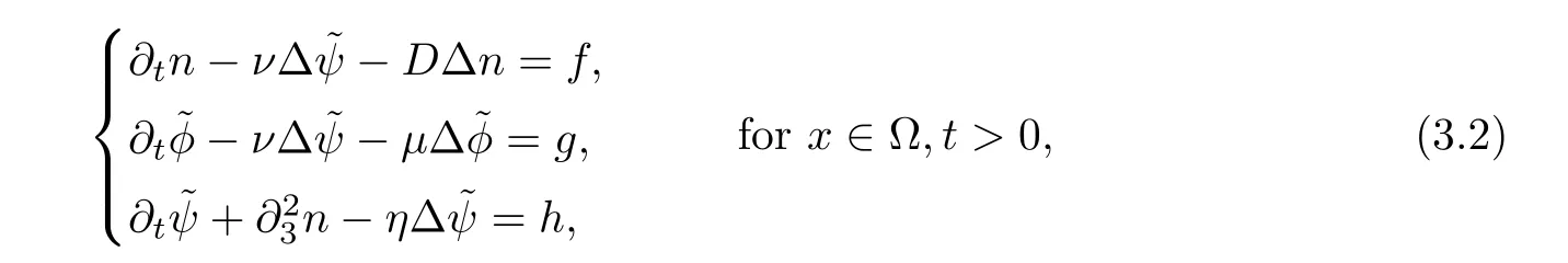
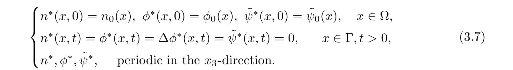
with the following initial and boundary conditions
The following two lemmas can be easily proved;see[8].
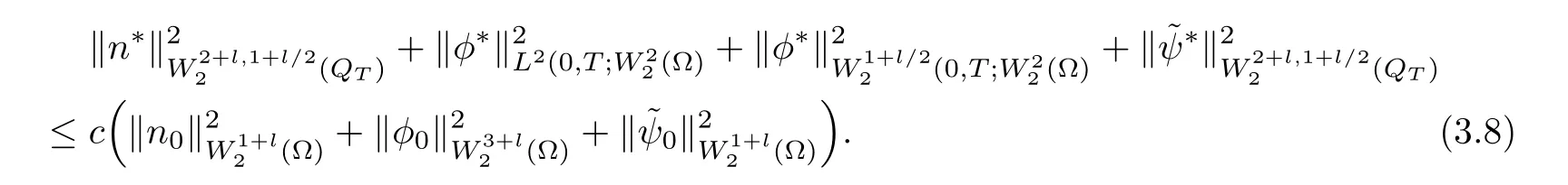
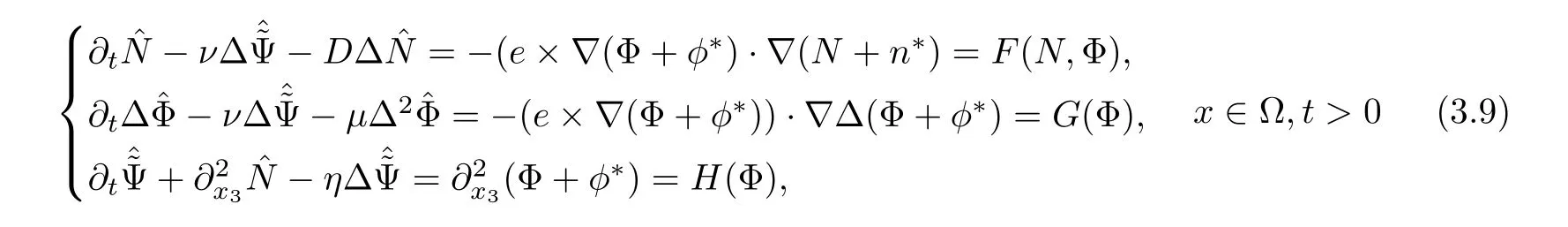
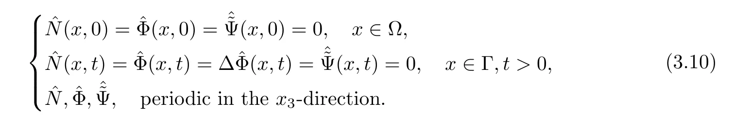
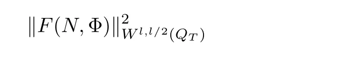
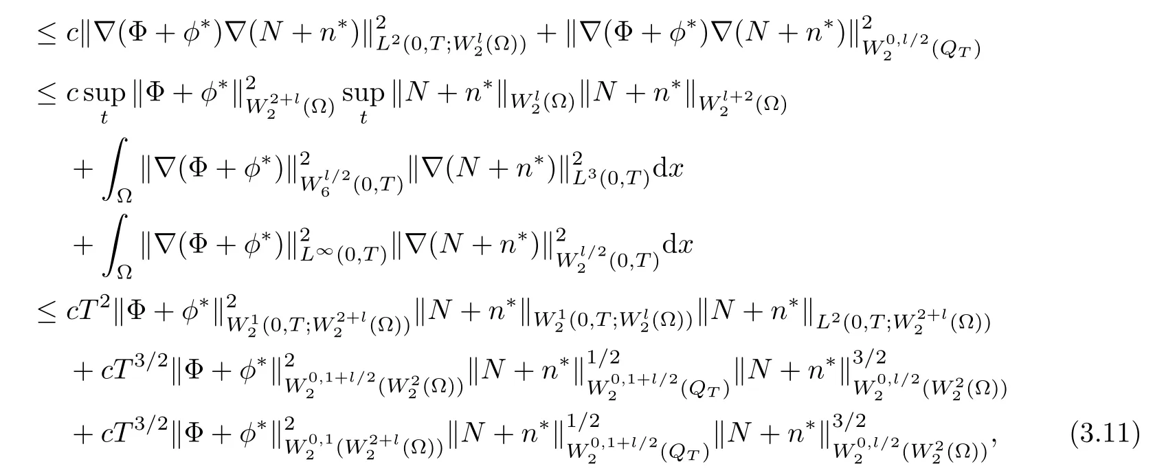
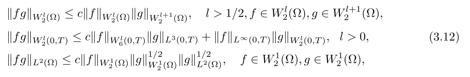
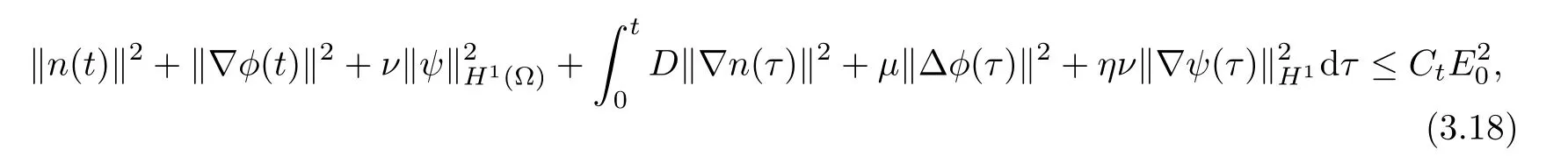
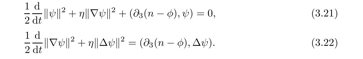
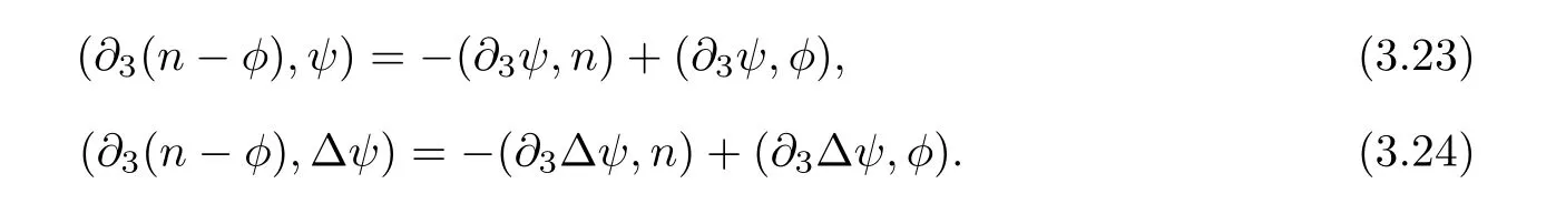
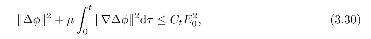
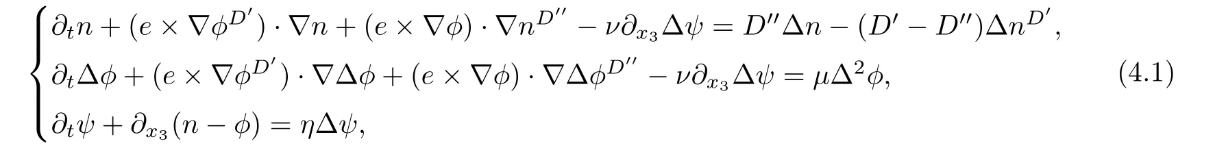
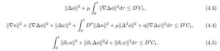
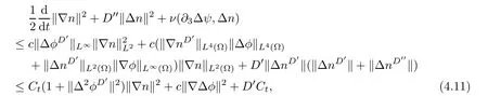
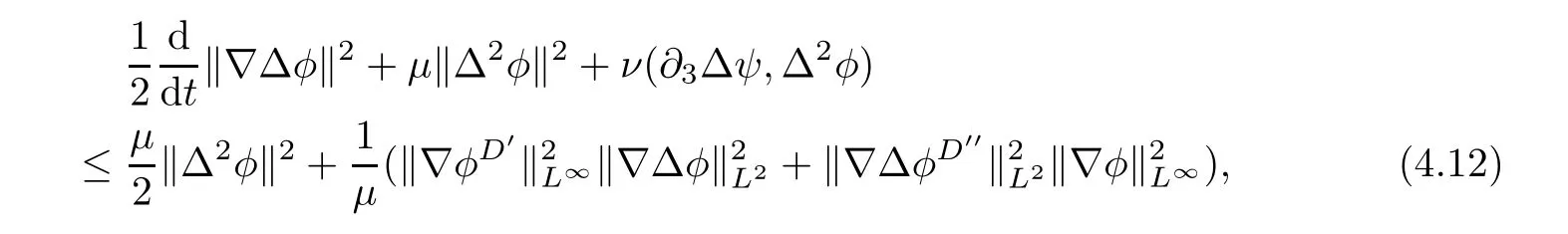
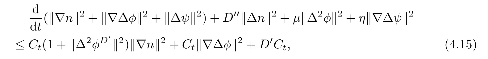
Lemma 3.1Let l≥0,D>0,μ>0,η>0 satisfy Dη> ν and 0 Lemma 3.2Let l>0 and assume thatthen there exists a unique solutionsuch thatin QTsatisfying the boundary conditions φ(x,t)=0 for x ∈ Γ,t>0 and periodic in the x3-direction.Moreover,there holds the inequality According to the above two Lemmas 3.1 and 3.2,there exists a unique solutionsatisfying and the initial-boundary conditions Moreover,there holds the inequality In the following,we use iterative technique to prove the existence of local-in-time solution for system(1.3).For this,letand consider the following linear system for and the initial-boundary conditions Hence,the existence of a solution for(1.3)inis equivalent to the existence of a fixed point of the solution mapdetermined by(3.10).This is achieved by the Banach fixed point theorem. Let BM?XTbe a ball of radius M to be determined later.The following proof is divided into three steps.First,we will show thatfor(N,Φ,Ψ)∈BM.Therefore,by Lemmas 3.1 and 3.2,there exists a solutionto(3.9)and(3.10)when the right hand side(F(Φ,N),G(Φ),H(Φ))is fixed byThen in the second step,we will show that the solution map F maps BMto itself for some M>0 and T′>0.Finally,in the third step,we will show that the mapping F is compressive and hence completes the proof of local existence of solutions in XTby Banach fixed point theorem. where(n?,φ?,ψ?)is estimated in(3.8).Here,we use the following calculus inequalities: and for any δ>0.This shows thatas long as Secondly,we show that the solution map F maps BMto itself for some M>0 and T?>0. Let Then from Lemmas 3.1 and 3.2,(3.11)and(3.14),it follows that Finally,we show the map is compressive.For this we considerandwhose solutions according to(3.9)and(3.10)areandrespectively.Then their differencesatisfies(3.9)with the right hand side replaced byH(Φ2))and the initial-boundary conditions.Then in a similar manner as that of(3.11)and(3.14),we obtain for any δ>0 and any t ∈ [0,T?].We can find positive small δ and T?? Therefore,it follows from Banach fixed point theorem that there exists a unique solution Considering the above local existence theory,we need only to obtain some a priori estimates of the solution(n,φ,ψ)for(1.3)to extend the solution to infinity.For simplicity,we only provide the formal estimates.Let T>0 be arbitrarily given. Lemma 3.3For any t∈[0,T],there exists some constant Ctdepending on t but independent of D such that ProofTake the L2inner product of the first equation in(1.3)with n to obtain Taking into account of the boundary conditions in(1.4),then by integration by parts,we obtain the last term on the left vanishes.Take the L2inner product of the second equation of(1.3)with φ to obtain Also,the last term vanishes by integration by parts because of the boundary conditions in(1.4).Taking the L2inner product of third equation of(1.3)with ψ and ?ψ,we obtain Taking into account of boundary conditions in(1.4),we obtain By adding(3.19),(3.20),(3.21)and(3.22)multiplied by ν ,and using H?lder inequality to(3.23),we obtain From this,(3.18)follows from Gronwall inequality. Lemma 3.4For any t∈[0,T],there exists some constant Ctdepending on t but independent of D such that ProofBefore giving the estimates,we first note that by the boundary conditions in(1.4),(e× ?φ)·? is a tangential derivative on Γ,and hence it follows from(1.3)that We take L2inner product of the second equation of(1.3)with?φ to obtain By virtue of integration by parts and H?lder inequality,we obtain Integrating this inequality over in yields for some constant Ctindependent of D,thanks to(3.18).By taking L2inner product of the first equation of(1.3)with?n,we obtain By integration by parts and the boundary conditions in(1.4),the last term vanishes.Similarly,by taking?to the third equation of(1.3)and then taking L2inner product with?ψ,we obtain In view of the boundary conditions in(3.27),we obtain by integration by parts Adding(3.31)and(3.32)multiplied by ν ,we obtain,by H?lder inequality, Integrating in time over[0,t],we obtain(3.26)with the help of(3.30). Lemma 3.5For any t∈[0,T],there exists some constant Ctdepending on t but independent of D such that ProofTake the L2inner product of the second equation of(1.3)with ?2φ to obtain By Young’s inequality,Gagliardo-Nirenberg inequalities,and Sobolev embedding theorem,we obtain and It then follows from(3.36)that because of(3.18)and(3.26).Therefore,we have,by Gronwall inequality, where Ctis a constant possibly depending on ν,μ,and η,but independent of D. Taking?to the third equation of(1.3)and then taking L2inner product of the first equation of(1.3)with?n,we obtain because of the boundary conditions in(3.27).In view of the Gagliardo-Nirenberg interpolation inequality,Sobolev embedding theorem,and(3.40)and(3.26),the right hand side can be bounded by Taking? to the third equation of(1.3)and then taking L2inner product with?2ψ,we obtain Adding(3.41)and(3.43)multiplied by ν ,with the help of H?lder inequality and(3.40),we obtain Integrating this inequality in time over[0,t]yields(3.35)for some constant Ctindependent of D. Lemma 3.6For any t∈[0,T],there exists some constant Ctdepending on t but independent of D such that ProofWe take?to the second equation of(1.3)and then take inner product with?2φ to obtain By integration by part,we obtain and with the help of(3.35) Therefore,we have Applying Gronwall inequality over[0,t]then yields the estimates(3.45). Then by standard arguments and using Lemmas 3.3,3.4,and 3.5,the solution(n,φ,ψ)can be extended to any time interval[0,T],hence completing the proof of Theorem 1.4.We also note that the uniqueness follows easily. In this section,we consider the vanishing diffusion limit as D→0.For fixedμ>0 and η >0,the estimates in Lemmas 3.3 to 3.6 hold uniformly in D.Let(nD,φD,ψD)be the solution obtained in Theorem 1.4.In what follows,we prove Theorem 1.5 by showing that(nD,φD,ψD)is a Cauchy sequence as D → 0 infollowing the argument because of Kato[7].Letandandbe two solutions of(1.3)with the same initial-boundary conditions in(1.4).Then,satisfies with homogeneous initial-boundary conditions(1.4)with(n0,φ0,ψ0)replaced with(0,0,0). Lemma 4.1Letthen there exists some constant Ctindependent of D′and D′′such that for any T>0, Proof(1)First,we obtain the zeroth order estimates.We multiply the first equation of(4.1)with n to obtain via integration by parts Taking the second equation in(4.1)with φ,then using integration by parts,H?lder inequality,and the Sobolev embedding theorem to obtain Taking inner product of third equation of(4.1)with(1??)ψ,we obtain Adding(4.6),(4.7),and(4.8)multiplied by ν ,we obtain,by H?lder inequality and Sobolev embedding theorem, where Ctis some constant independent of D′and D′.It is standard from Gronwall inequality that(4.2)holds for any T>0. Then,by taking inner product of the second equation of(4.1)with?φ,we obtain Integrating this inequality in time over[0,t]and using(3.26)and(4.2),we obtain(4.3). (2)We establish first order estimates.Take the inner product of the first equation of(4.1)with?n,then we obtain,by integration by parts and homogeneous boundary conditions, because of Sobolev embedding theorem and(3.35).Take the L2-inner product of the second equation of(4.1)with ?2φ to obtain from which it follows that because of(3.35)and Sobolev embedding theorem.Take?to the third equation of(4.1)and then take the L2-inner product with?ψ to obtain Adding(4.11),(4.13),and(4.14)multiplied by ν,we obtain from which it follows(4.4)by Gronwall inequality. (3)We establish the time derivative estimates.By the estimates in the above two parts,we immediately have(4.5). AcknowledgementsThis work was finished when the first author was visiting the Institute of Applied Physics and Computational Mathematics.The first author wish to thank the hospitality of the Institute of Applied Physics and Computational Mathematics.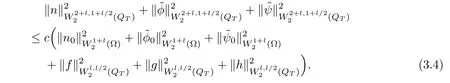


3.2 A priori estimates


4 Vanishing Diffusion Limit


 Acta Mathematica Scientia(English Series)2020年2期