k-NORMAL DISTRIBUTION AND ITS APPLICATIONS

HAN Tian-yong,WEN Jia-jin,SONG An-chao,YE Jian-hua

(1.College of Information Science and Engineering,Chengdu University,Chengdu 610106,China)(2.School of Statistics,Southwestern University of Finance and Economics,Chengdu 611130,China)

k-NORMAL DISTRIBUTION AND ITS APPLICATIONS

HAN Tian-yong1,WEN Jia-jin1,SONG An-chao2,YE Jian-hua1

(1.College of Information Science and Engineering,Chengdu University,Chengdu 610106,China)(2.School of Statistics,Southwestern University of Finance and Economics,Chengdu 611130,China)

In this paper,we study the truncated variables andk-normal distribution.By using the theory of logarithmic concave function,we obtain the inequality chains involving variances of truncated variables and the function of truncated variables,which is the generalization of some classical results involving normal distribution and the hierarchical teaching model.Some simulation results and a real data analysis are shown.

truncated random variables;k-normal distribution;hierarchical teaching model;logarithmic concave function;simulation

1 Introduction

With the expansion of university enrollment,various work to improve students’ability all round was continued to be carried out.How to increasingly improve teaching quality in the courses with large number of students(such as advanced mathematics)are discussed repeatedly.Since the examination scores of the large number of students obey normal distribution,statistical theory is a natural research tool for study of a large scale teaching(see[1,2]).

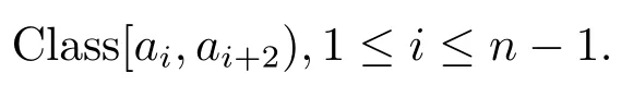
The math score of the students of some grades in a university is a random variableξI,whereξI∈I=[0,100).Assume that the students are taught by divided intonclasses according to their math scores,written as：Class[a1,a2),Class[a2,a3),···,Class[an,an+1),wheren≥ 3,0=a1＜a2＜···＜an+1=100,andai,ai+1are the lowest and the highest math scores of the students of the Class[ai,ai+1),respectively.This model of teaching is called hierarchical teaching model(see[1-4,7]).This teaching model is often used in college English and college mathematics teaching.In teaching practice,the previously mentioned score maybe the math score of national college entrance examination or entrance exams which represent the mathematical basis of the students,or in mathematical language,the initial value of the teaching.

No doubt that this teaching model is better than traditional teaching model.However,the real reason for it’s high efficiency and the further improvement are not found.As far as we know,not many papers were published to deal these since the difficulty of computing the inde fi nite integrals involving the normal distribution density function.In[3],by means of numerical simulation,the authors proved the variance of the hierarchical class is smaller.In[4],the authors established some general properties of the variance of the hierarchical teaching,and established a linear model of teaching efficiency of hierarchical teaching model.If the students are divided into Superior-Middle-Poor three classes,the authors believe that the three classes,especially the third one will bene fi t most from the hierarchical teaching.

In order to study the hierarchical teaching model,we need to give the de fi nition of truncated variables.

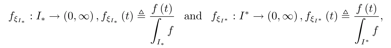
De fi nition 1.1LetξI∈Ibe a continuous random variable,and let its probability density function(p.d.f.)bef：I→(0,∞).IfξI?∈I??Iis also a continuous random variable and its probability density function is

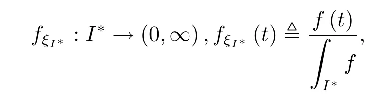
then we call the random variableξI?a truncated variable of the random variableξI,denoted byξI??ξI;ifξI??ξI,andI??I,then we call the random variableξI?a proper Truncated Variable of the random variableξI,denoted byξI??ξI,hereI,I??(-∞,∞),IandI?are intervals.

In the hierarchical teaching model,the math score of Class[ai,ai+1)is also a random variableξ[ai,ai+1)∈[ai,ai+1).Since[ai,ai+1)?I,we say it is a proper truncated variables of the random variableξI,written asξ[ai,ai+1)?ξI,i=1,2,···,n.Assume that Class[ai,ai+1)and Class[ai+1,ai+2)are merged into one,i.e.,

Since[ai,ai+1)?[ai,ai+2)and[ai+1,ai+2)?[ai,ai+2),we know thatξ[ai,ai+1)andξ[ai+1,ai+2)are the proper truncated variables of the random variableξ[ai,ai+2).

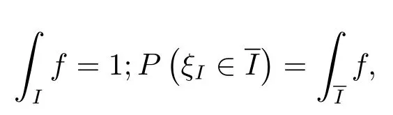
We remark here ifξI∈Iis a continuous random variable,and its p.d.f.isf：I→(0,∞),then the integrationfconverges,and it satis fi es the following two conditions

According to the de fi nitions of the mathematical expectationEξI?and the varianceDξI?(see[8,9])with De fi nition 1.1,we are easy to get

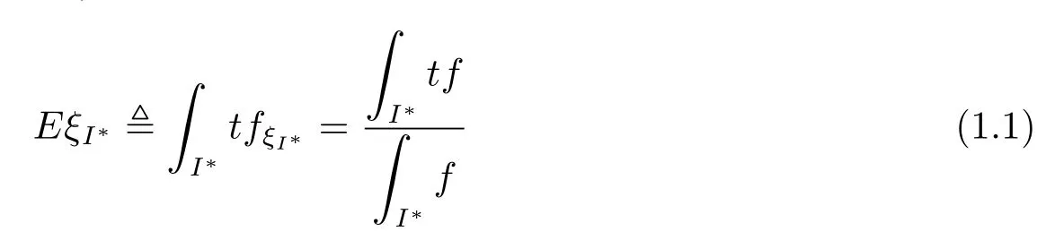
and

whereξI?is a truncated variable of the random variableξI.

In the hierarchical teaching model,what we concerned about is the relationship between the variance ofξ[ai,ai+1)and the variance ofξI,wherei=1,2,···,n.Its purpose is to determine the superiority and inferiority of the hierarchical teaching model and the traditional mode of teaching.If

then we believe that the hierarchical teaching model is better than the traditional mode of teaching.Otherwise,we believe that the hierarchical teaching model is not worth promoting.

2 k-Normal Distribution

The normal distribution(see[3,4,8,9])is considered as the most prominent probability distribution in statistics.Besides the important central limit theorem that says the mean of a large number of random variables drawn from a common distribution,under mild conditions,is distributed approximately normally,the normal distribution is also tractable in the sense that a large number of related results can be derived explicitly and that many qualitative properties may be stated in terms of various inequalities.

One of the main practical uses of the normal distribution is to model empirical distributions of many di ff erent random variables encountered in practice.For fi t the actual data more accurately,many research for generalizing this distribution are carried out.Some representative examples are the following.In 2001,Armando and other authors extended the p.d.f.to the normal-exponential-gamma form which contains four parameters(see[5]).In 2005,Saralees generalized it into the formKexp(see[6]).In 2014,Wen Jiajin rewrote the p.d.f ask-Normal Distribution as follows(see[7]).

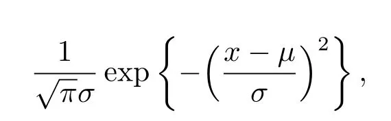
De fi nition 2.1Ifξis a continuous random variable and its p.d.f.is

then we call the random variableξfollows thek-normal distribution,denoted by,whereμ∈(-∞,∞),σ∈(0,∞),k∈(1,∞),anddxis the gamma function.

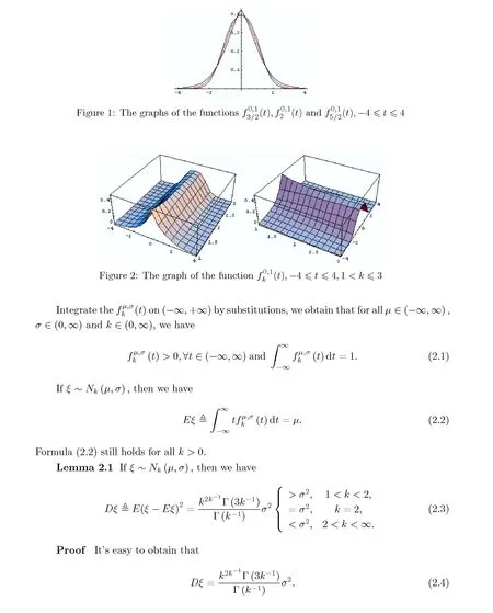
By the graph of the functionω(k)(depicted in Figure 3),we know that the functionis monotonically increasing.Hence the functionis monotonically decreasing.Note thatω?(2)=1,we get

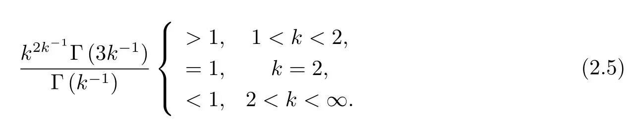
Using(2.4)and(2.5),we get our desired result(2.3).

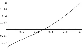
Figure 3：The graph of the functionω(k),0＜k＜1

According to the previous results,we fi nd thatk-normal distribution is a new distribution similar to but di ff erent from the normal distribution and the generalized normal distribution(see[5,6]),it is also a natural generalization of the normal distribution,and it can be used to fi t a number of empirical distributions with di ff erent skewness and kurtosis as well.

We remark here thatk-normal distribution has similar but distinct form to the generalized normal distribution in[6].By De fi nition 2.1,we know thatis the p.d.f.of normal distributionN(μ,σ).But the p.d.f.fors=2(in[6])is

which does not match with normal distribution.So,to a certain extent,k-normal distribution is a better form of the generalized normal distribution.

3 Main Results

In this section,we will study the relationship among the variances of truncated variables.The main result of the paper is as follows.

Theorem 3.1Let the p.d.f.f：I→(0,∞)of the random variableξIbe di ff erentiable,and letDξI?,DξI?,DξIbe the variances of the truncated variablesξI?,ξI?,ξI,respectively.If

(i)f：I→(0,∞)is a logarithmic concave function;

(ii)ξI??ξI,ξI??ξ,I??I?,

then we have the inequalities

Before prove Theorem 3.1,we fi rst establish the following three lemmas.

Lemma 3.1LetξI∈Ibe a continuous random variable,and let its p.d.f.bef：I→(0,∞).IfξI??ξI,ξI??ξI,I??I?,then we have

ifξI??ξI,ξI??ξI,I??I?,then we have

ProofBy virtue of the hypotheses,we get

thus

It follows therefore from the above facts and De fi nition 1.1 that we have

Lemma 3.2Let the functionf：I→(0,∞)be di ff erentiable.Iffis a logarithmic concave function,then we have

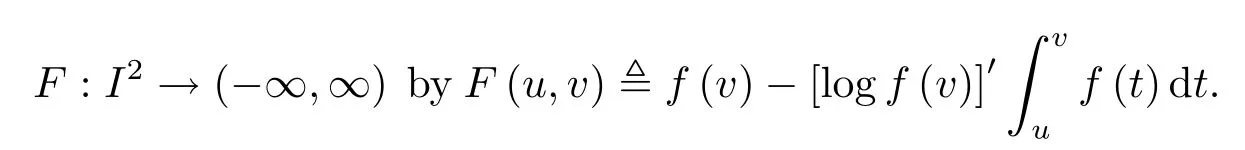
ProofWe define an auxiliary functionFof the variablesuandvas

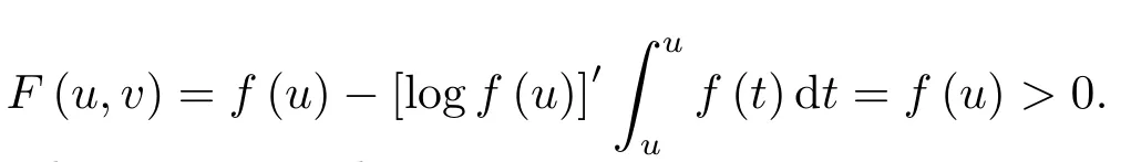
Ifv=u,then we have

By Cauchy mean value theorem,there exists a real numberθ∈(0,1)forsuch that

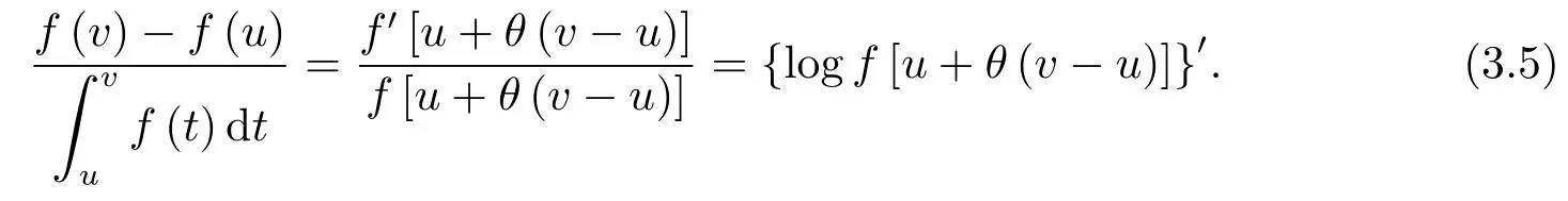
Ifu＜v,then we have

Combining(3.5)and(3.6),we obtain

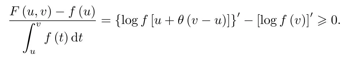
SoF(u,v)≥f(u)＞0.This proves inequality(3.4)foru＜v.

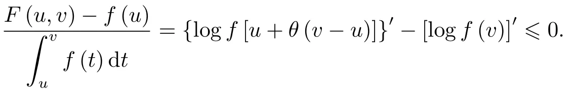
Ifu＞v,then we have

Combining(3.5)and(3.7),we obtain

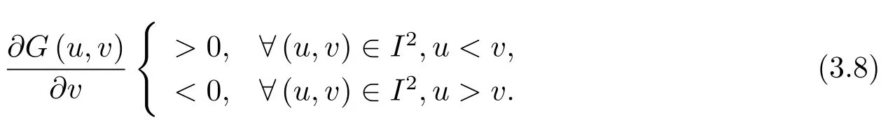
Lemma 3.3Let the functionf：I→(0,∞)be di ff erentiable.Iffis a logarithmic concave function,then the function

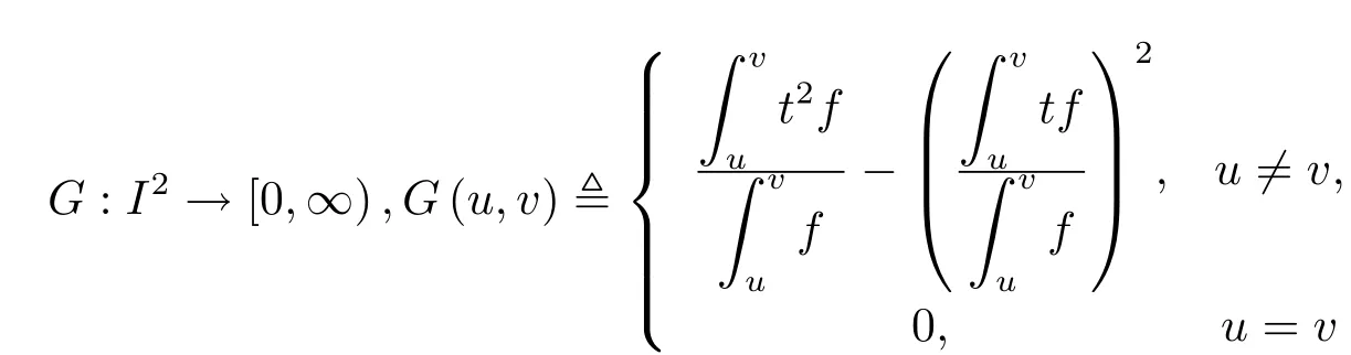
satis fi es the following inequalities

ProofFor the convenience of notation,two real numbers with same signαandβwill be written as.

By the de fi nition,we know that

The power mean inequality asserts(see[10])that

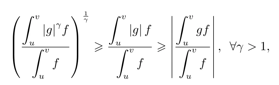
then we are easy to get

where

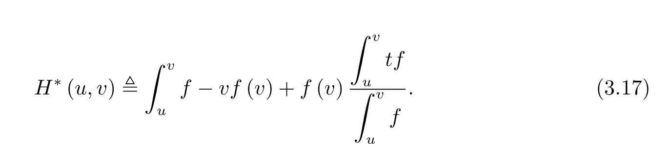
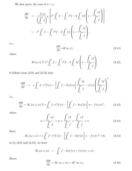
Combining(3.9),(3.14),(3.17),v＞uwith Lemma 3.2,we can do the straight calculation as follows

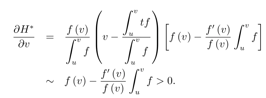
By(3.17)andv＞u,we get

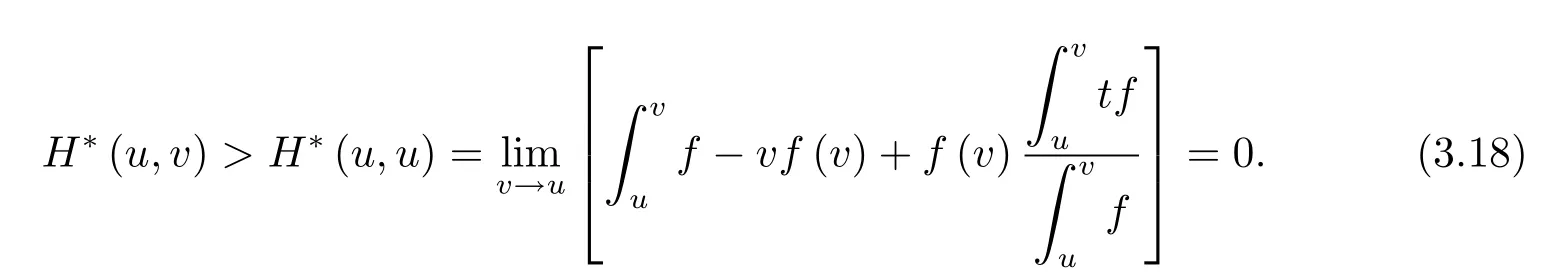
By(3.16)and(3.18),we get

By(3.19)andv＞u,we get

From(3.11)and(3.20),for the case ofv＞u,result(3.8)of Lemma 3.3 follows immediately.

Next,we prove the case ofu＞v.Based on the above analysis,we obtain the following relations

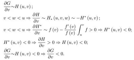
Thus inequalities(3.8)still hold foru＞v.This completes our proof.

Now we turn our attention to the proof of Theorem 3.1.

ProofWithout loss of generality,we can assume that

Note that

Ifα≤a＜b＜β,so according to(1.2),(3.10)and Lemma 3.3,we get

hence

Ifα＜a＜b≤β,so,according to(1.2),(3.10)and Lemma 3.3,we get

That is to say,inequality(3.21)still holds.

By Lemma 3.1,we haveξI??ξI,ξI??ξI,I??I??ξI??ξI?.Using inequality(3.21)forξI?,ξI?,we can obtain

Combining inequalities(3.21)and(3.22),we get inequalities(3.1).

This completes the proof of Theorem 3.1.

From Theorem 3.1 we know that if the probability density function of the random variableξIis di ff erentiable and log concave,andξI?is the proper truncated variables of the random variableξI?,the variance ofξI?is less than the variance ofξI?.This result is of great signi fi cance in the hierarchical teaching model,see the next theorem.

For the convenience of use,Theorem 3.1 can be slightly generalized as follows.

Theorem 3.2Letφ：I→(-∞,∞)andf：I→(0,∞)be di ff erentiable functions,wherefbe the p.d.f.of the random variableξI,and letDφ(ξI?),Dφ(ξI?)withDφ(ξI)be the variances of the truncated variablesφ(ξI?),φ(ξI?)withφ(ξI),respectively.If

(i)φ′(t)＞0,?t∈I;

(ii)the function(f? φ-1)(φ-1)′：φ(I)→(0,∞)is log concave;

(iii)ξI??ξI,ξI??ξI,I??I?,

then we have the following inequalities

ProofSet.By condition(i),we can see that0 and

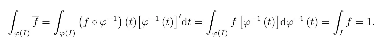
By condition(ii),we can see thatis a logarithmic concave function.Combining conditions(i)and(iii)with Lemma 3.1,we have

We can deduce from Theorem 3.1 that the following is true

Thus inequalities(3.23)is valid.

4 Applications

In the hierarchical teaching model,the math score of the students of some grade in a university is a random variableξI,whereI=[0,100),ξI?ξ,ξ∈(-∞,∞).By using the central limit theorem(see[8]),we know thatξfollows a normal distribution,that is,2(μ,σ).If,in the grade,the top students and poor students are few,that is to say,the varianceDξof the random variableξis small,according to Figure 1 and Figure 2 with Lemma 2.1,we believe that there is a real numberk∈[2,∞)such that(μ,σ).Otherwise,there is a real numberk∈(1,2)such that(μ,σ).Then thek，σofNk(μ,σ)can be determined according to[5].

We have collected three real data setsX1,X2 andX3,which are all math test score of the students from the unhierarchical,the fi rst level(superior)and the second level(poor)classes,containing 263,149 and 145 records,respectively.For further analyzing the data,we fi rst estimate parametersk，μ，σofNk(μ,σ),then draw probability density function ofNk(μ,σ)and frequency histogram of the corresponding data set in the same coordinate system,which also contains the probability density function curve graph of normal distribution.After that,we obtain three graphs forX1,X2 andX3,respectively(see Figure 4,Figure 5 and Figure 6 in Appendix B).These three fi gures show thatk-normal distribution is superior to normal distribution since kurtosis is bigger and variance is smaller.

Further more,as shown in the histograms,the variance ofX1,X2 andX3 is decreasing.By observing the proportion of scores less than 60 ofX1,X2 andX3,we fi nd that the hierarchical teaching model bring better results,and that the second category(represented byX3)classes receive more signi fi cant bene fi ts from this teaching model.

According to Theorem 3.1 and Lemma 2.1,we have

Theorem 4.1In the hierarchical teaching model,if(μ,σ),wherek＞1,then for alli,n：1≤i≤n-1,n≥3,we have

where

We accomplish simulation analysis about Theorem 3.1.The procedure of simulation design is shown in Appendix A.The results of the simulation are listed in the tables(see Tables 1-4 in Appendix A).By comparing the data in these tables,we fi nd that,no matter how to change the parametersk，μorσ,the variance of truncated variable is strictly less than that of untruncated variable.For example,for anyk,μorσas shown in Tables 1-4,

this does verify the truth of Theorem 3.

From Tables 1 and 3,we see that for eachσandI?(-∞,∞),if

thenDξ1I＜Dξ2I＜Dξ3I.From Tables 2 and 4,for eachμandI?(-∞,∞),if

thenDη1I＜Dη2I＜Dη3I.The truth of Theorem 3.1 is verified.

Actually in appendix,the data set X1 is the math test score of unhierarchical students,X2 and X3 are math test score of hierarchical students.We have fi gured out their variances

The factsD(X3)＜D(X1)andD(X2)＜D(X1),just show that the hierarchical teaching is more efficiency than unhierarchical teaching.

[1]Yao Hui,Dai Yong,Xie Lin.Pareto-geometric distribution[J].J.Math.,2012,32(2)：339-351.

[2]Deng Yuhui.Probablity distribution of sample spacing[J].J.Math.,2004,24(6)：685-689.

[3]Yang Chaofeng,Pu Yingjuan.Bayes analysis of hierarchical teaching[J].Math.Prac.The.(in Chinese),2004,34(9)：107-113.

[4]Han Tianyong,Wen Jiajin.Normal distribution and associated teaching efficiency[J].Math.Prac.The.(in Chinese).2014,44(6)：183-193.

[5]Armando D,Graciela G,Ramon M.A practical procedure to estimate the shape parameter in the generalized Gaussian distribution,technique report[OL].Available：http：//www.cimat.mx/reportes/enlinea/I-01-18 eng.pdf,2001.

[6]Saralees N.A generalized normal distribution[J].J.Appl.Stat.2008,32(7)：685-694.

[7]Wen Jianjin,Han Tianyong,Cheng S S.Quasi-log concavity conjecture and its applications in statistics[J].J.Inequal.Appl.,2014,DOI：10.1186/1029-242X-2014-339.

[8]Johnson O.Information theory and the central limit theorem[M].London：Imperial College Press,2004.

[9]Wlodzimierz B.The normal distribution： characterizations with applications[M].New York：Springer-Verlag,1995.

[10]Wang Wanlan.Approaches to prove inequalities(in Chinese)[M]Harbin：Harbin Institute of Technology Press,2011.

[11]Tong T L.An adaptive solution to ranking and selection problems[J].Ann.Stat.,1978,6(3)：658-672.

[12]Bagnoli M,Bergstrom T.Log-concave probability and its applications[J].Econ.The.,2005,26(2)：445-469.

Appendix

A The Simulation and Comparison of Variances of Truncatedk-Normal Variable

The procedure of simulation design is as follows

Step 1Choose the appropriate parameterk,μandσin the distributionNk(μ,σ);

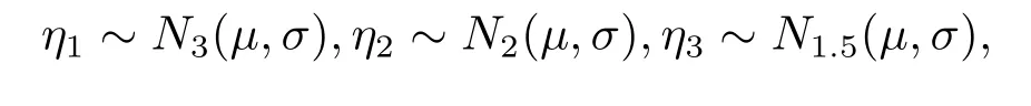
Step 2Generate 200 random numbers obeying the distribution(μ,σ);

Step 3Use the 200 numbers to calculate the variance for six truncatedk-normal variablesξ(-∞,∞),ξ[0,60),ξ[60,80),ξ[80,100),ξ[0,80)andξ[60,100);

Step 4Repeat Step 1 and Step 2 for 50 times;

Step 5Calculate the mean of 50 variances for each truncatedk-normal variable，denoted byDξ(-∞,∞),Dξ[0,60),Dξ[60,80),Dξ[80,100),Dξ[0,80)andDξ[60,100)respectively;

Step 6Change the value ofk,μandσ,and repeat Step 1,Step 2,Step 3,Step 4.All the results are listed in Tables 1-4(NaN indicates there is no random number for corresponding truncated variable).

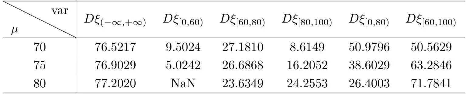
Table 1：k=3,σ=10

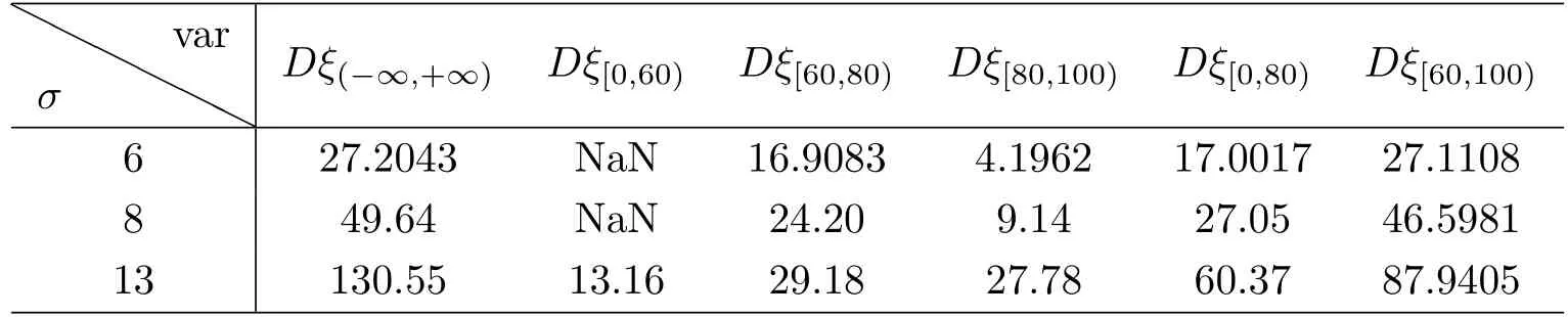
Table 2：k=3,μ=75

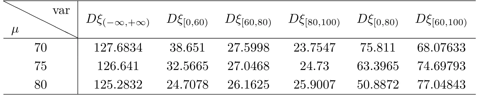
Table 3：k=1.5,σ=10

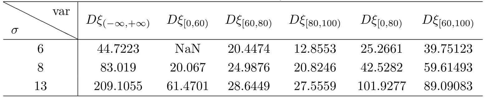
Table 4：k=1.5,μ=75

B Curve Fitting for Three Real Data SetsX1,X2andX3

The results of curve fi tting for three real data sets are as follows(see Figure 4-6)

k-正態(tài)分布及其應(yīng)用

韓天勇1,文家金1,宋安超2,葉建華1

(1.成都大學(xué)信息科學(xué)與工程學(xué)院,四川成都 610106)(2.西南財(cái)經(jīng)大學(xué)統(tǒng)計(jì)學(xué)院,四川成都 611130)

近本文研究了截?cái)嚯S機(jī)變量和k-正態(tài)分布.利用對(duì)數(shù)凹函數(shù)理論,獲得了涉及截?cái)嚯S機(jī)變量和截?cái)嚯S機(jī)變量的函數(shù)的方差的不等式鏈,推廣了涉及正態(tài)分布和分層教學(xué)模型的一些經(jīng)典結(jié)論.同時(shí)在附錄部分給出了仿真結(jié)果.

截?cái)嚯S機(jī)變量;k-正態(tài)分布;分層教學(xué)模型;對(duì)數(shù)凹函數(shù);仿真

O174.13;O211.3;O211.5

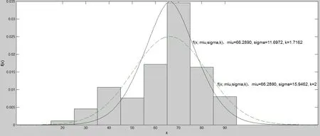
Figure 4：FittingX1

Figure 5：FittingX2

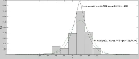
Figure 6：FittingX3

on：62J10;62P25;60E05;60E15;26D15;26E60

A Article ID： 0255-7797(2017)04-0737-14

date：2016-02-25Accepted date：2016-09-28

Supported by the Natural Science Foundation of Sichuan Science and Technology Department(2014SZ0107).

Biography：Han Tianyong(1976-),male,born at Chengdu,Sichuan,associate professor,major in dynamical system,inequality and its application.

MR(2010)主題分類(lèi)號(hào)：62J10;62P25;60E05;60E15;26D15;26E60