The effect of simple imputation on inferences about population means when data are missing in biomedical research due to detection limits

Hongyue WANG*, Guanqing CHEN Xiang LU Hui ZHANG, Changyong FENG3

?Biostatistics in psychiatry (29)?

The effect of simple imputation on inferences about population means when data are missing in biomedical research due to detection limits

Hongyue WANG1,*, Guanqing CHEN1, Xiang LU1, Hui ZHANG2, Changyong FENG1,3

sample geometric mean; population geometric mean; two-sample test

1. Introduction

Detection limit is a long standing problem in experimental sciences. It refers to the limited ability of an instrument in measuring an outcome of interest in a certain range (typically small values close to 0). Many instruments cannot return meaningful measurements if signals fall below a certain threshold value. This problem is especially prevalent in biomedical sciences as signals are sometimes too weak to be detected in the presence of ambient noise. Although detection limits are often due to limitations of physical devices, the problem may also arise in psychosocial research with assessments based on instruments (questionnaires). For example, in alcohol and substance use research, alcohol or drug use may not be detected in a subject if the blood level is not sufficiently high. Also, if answers for all or most subjects to an item in a questionnaire fall below (or above) a certain score in the potential range of scores, the lack of variability in the outcome may prevent any useful analysis of the data.

Detection limit presents problems for statistical analysis since no data (or very little data) is observed in part of the potential range of the variable. It is not possible to gauge the variability of the outcome below the detection limit, but this information is needed to conduct standard statistical inference on the data in the whole range (for example, to estimate the geometric mean of the population from which the sample is drawn). A commonly used ad-hoc method to deal with this problem is to impute data below the detection limit and then apply standard statistical methods.[1]This practice is especially prevalent in biomedical research.Geometric means are the most popular method of imputing values below the detection limit because data are often log-transformed to reduce skewness before being analyzed (even though the log-transformation may not actually reduce the skewness[2]). The arithmetic mean of the log-transformed outcome is the logarithm of the sample geometric mean.

Although imputation seems natural and intuitive,it has significant implications for statistical inference and, thus, on the reported results of research.[3,4]In this report we discuss the pitfalls of using this common method of imputation in research and in clinical practice.

2. Geometric mean of a non-negative random variable

The so-called ‘geometric mean’ used in biomedical and psychosocial research is actually the sample geometric mean, that is, the geometric mean of a sample of observations from an underlying distribution.

For example, let ai, i=1,...,n, be a sequence of non-negative numbers; then the geometric mean of the sequence isThis is what is commonly referred to as the ‘geometric mean’, but it is important to keep in mind that the sample and population means are completely different concepts. The former is computable based on the sample, while the latter is an unknown quantity, or a parameter in the nomenclature of statistics. The geometric mean described above is actually a sample geometric mean because it is a computable quantity. Unlike the arithmetic, the population geometric mean had never been clearly defined in the literature until the recent work of Feng and colleagues[2,3]who presented a formal definition of this elusive quantity. The population geometric mean of a non-negative variable X defined if either X has non-zero probability at zero (that is, X may equal 0) or X is positive with |log X| having a finite mean value,that is, E|log X|<∞ . Subsequently the definition was further broadened to only require that E|log X| exists(which includes E|log X|<∞ as a special case) and the properties of the population geometric mean were elaborated.[4]This work lays a conceptual foundation to interpret the sample geometric mean (as an estimate of the underlying population geometric mean) and clarifies some ambiguities in using the geometric mean in biomedical research. A brief summary of this work is shown in Box 1.

The geometric mean has a very unusual property.We know that for a positive random variable, arithmetic mean, if it exists, is always positive. However, for some positive random variables, geometric means can be zero. This fact is counterintuitive as the sample geometric mean obtained from a positive random variable is always positive. This unusual property can have significant implications for inference about the population geometric mean when the data in the sample is left-censored due to a detection limit.

Another issue is the relationship between the geometric mean and the arithmetic mean for a positive random variable. In biomedical research, data is often right-skewed with most values close to the lower limit.A popular approach for dealing with this is to logtransform the data, analyze the transformed data, and then transform the result back to the original scale.For a non-negative random variable X, in general there is no connection between the geometric mean GMXand the arithmetic mean E(X), even if they both exist.For example, for two log-normally distributed random variables, if they have the same log-mean values but different log-variances, then their geometric means are equal but their arithmetic means are not equal. This means that we cannot test the hypothesis that they have the same (arithmetic) mean values by testing that the log-transformed data have the same (arithmetic)mean values. This fact is not well appreciated in biomedical research.[2]

BOX 1. Relationship of population and sample geometric means

? Suppose F(x) is the probability distribution function of a non-negative random variable X. If F(0) ＞ 0,then the geometric mean of X, denoted by GMX, is defined as 0. If X is positive and the expected value of|log X| exists, then we define GMXas exp(E log X). If F(0)≠0 and the expected value of |log X| does not exist, then it is not possible to define the geometric mean of X. Hence, we cannot define the geometric mean for all non-negative random variables, just like the mean cannot be defined for all random variables. However, if GMXis well defined, it is the population geometric mean, which can be used to interpret the sample geometric mean of X.

? Suppose the geometric mean of X exists, and, Xi, i=1,...,n is a random sample from the distribution of X. Letbe the sample geometric mean. Then the sample geometric mean is strongly consistent[3,4]and, thus, is a consistent estimate of the population geometric mean.

3. Geometric mean with detection limit

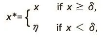
In this section, we discuss the effect of the na?ve imputation method on the geometric mean in the presence of a detection limit. Let X be a positive random variable and δ be the lower detection limit; X is unobservable(missing) if X < δ. A common approach in biomedical research is to define a modified version of X by:where η is some positive constant. Usually, η=δ/2, or a small positive constant less than δ.[1,5-15]After the imputation, inference about the population geometric mean of the original data proceeds by treating the imputed data as if they were observed.

To discuss potential effects of this naive imputation on inference about the population geometric mean, we assume that X is a positive random variable, which is the case in most real-study applications.

a) Case 1: GMX>0. The geometric mean of X* can be greater than, less than, or equal to GMXdepending on the distribution of X below the detection limit. If the detection limit δ is small enough, then with relatively large sample sizes inferences based on the imputed data (such as confidence intervals, the two-sample t-test,and the paired t-test) yield valid results for the original data. However, if δ is large, imputation may yield invalid results.

b) Case 2: GMX=0. With the imputation, the geometric mean of X* depends on how the imputed value η is selected and is always greater than η. This means that the estimated geometric mean based on the imputed data may be very far away from the theoretical geometric mean of zero. Another effect is that the imputation brings some arbitrariness into the statistical inference.

Thus whether GMX>0 or GMX=0, imputation has significant implications for inference about the population geometric mean. If GMX>0, inference using common statistical methods is reasonably robust if the detection limit is small; but if GMX=0, any analysis of the geometric mean based on the imputed data is invalid and the result is uninterpretable. Unfortunately,the detection limit makes it impossible to determine whether GMX>0 or GMX=0.

4. Simulation results

As described above, when the sample geometric mean of a positive random variable is 0, the geometric mean of the modified observation (which imputes values below the detection limit δ) may be very different from 0 and, thus, inferences based on the modified sample may be misleading.

Suppose Y has a standard log-normaldistributionwith its probability distribution function , and U is independent of Y and uniformly distributed on (0,1).Let C0be a positive constant. The random variable X is defined as:

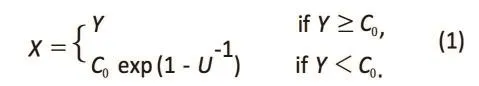
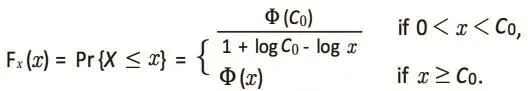
The distribution function of X is:

In the simulation study, C0is set at 0.277602. The data X1,…..,Xnis generated from the distribution of X defined in equation (1) above.

4.1 Properties of geometric mean

Figure 1 shows the cumulative distribution function of X and Y when C0=0.1. Since, it is nearly impossible to distinguish between the two distribution function curves in the figure. However, their geometric means are very different. It is easy to prove that GMY=1 and GMX=0, no matter how small C0is (see Example 2 in Feng and colleagues[4]for a proof).

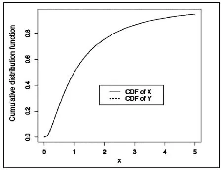
Figure 1. Cumulative distribution functions of X andY in formula (1) with c0=0.1

Since X is positive, the sample geometric mean is always positive. Although the sample geometric mean is a consistent estimator of GMX(which is 0 in this case), it may be quite a large number. Table 1 is a sample of n=100 observations from the distribution of Z=100X, where X is defined in equation (1). The sample geometric meanis. However, the population geometric mean is actually GMZ=0. It is very difficult to imagine that the data in Table 1 is from a distribution with a geometric mean of 0. This strange property of the geometric mean makes it difficult to test whether or not a sequence of positive numbers is a sample from a distribution with a geometric mean equal to 0.

In the simulation study, we set the detection limit at δ=0.277602 such that there was a 10% probability that Xiis below the detection limit, that is, Pr{X<0.277602}=0.1.No data is observed below this detection limit, so if the value of δ/2 is imputed for all cases in which Xifalls below δ=0.277602, then the modified observations are

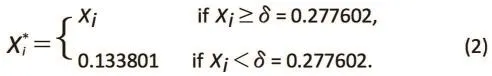
Table 2 shows the means and standard deviationsfor samples of different sizes after 100,000 Monte Carlo replications. In eachis generated,the mean and standard deviation ofmean and sample standard deviation based on 100,000 Monte Carlo replicates.

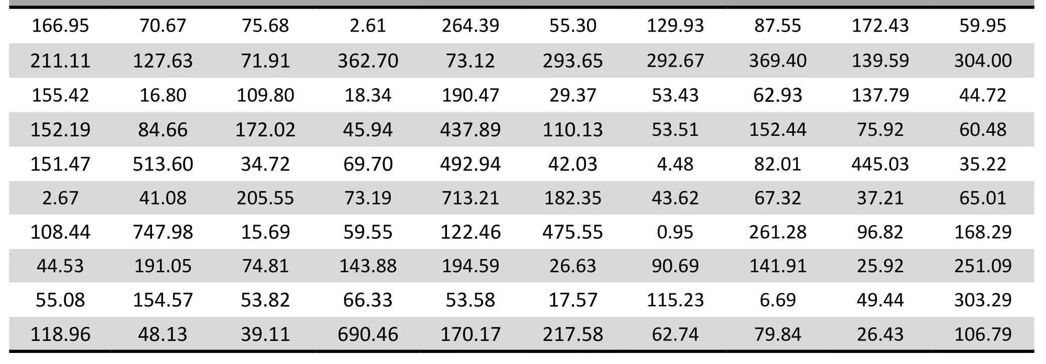
Table 1: A random sample from a distribution with geometric mean 0 (sample size n=100)

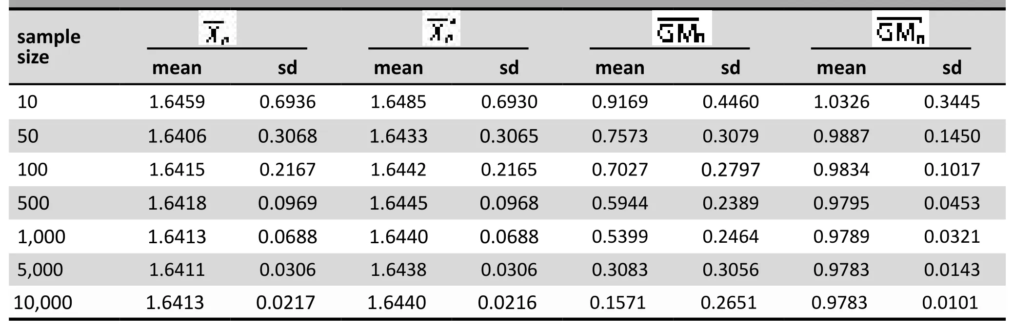
Table 2: Means and standard deviations of sample means and sample geometric means

Figure 2. Histogram of sample geometric means from the distributions of X (part A) and X* (part B) in formula (2) for different sample sizes

The same interpretation applies to the other columns in the table. There are two main findings shown in the table:

a) Since the detection limit is relatively small,the difference between the means and is very small. They are very close to E(X1) and E() even for small sample sizes.

4.2 Hypothesis testing using geometric means

Let X11, ..., X1,n1and X21, ..., X2,n2be be two independent samples. Suppose we want to test the hypothesis:H0: GMX11=GMX21.

Due to detection limit, only the modified data can be used. The test statistic used in biomedical research is of the form

In the simulation studies, X11has the same distribution as defined in equation (2) with c0=0.277602 and X21is defined as 2X11. Figure 3 shows the histograms of p-values of the test statistic T* for different sample sizes. In our example both samples have the same geometric means, so the null hypothesis is true and the distribution of the p-values of the statistic test T* should be close to the uniform distribution, at least for large sample sizes. However, the histograms shown in Figure 3 clearly indicate otherwise. Thus results of testing the null hypothesis when using the modified data are difficult to interpret and can be quite misleading.

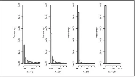
Figure 3. Histograms of p-values of the test statistic in formula (3) for different sample sizes

5. Discussion

In this paper we consider the effect of the most common method of data imputation used in biomedical research for results that are below a detection limit.Despite its popularity, this method of using imputed values to compute a sample geometric mean which is used to estimate the population geometric mean(needed in many common statistical analyses) has not been adequately reviewed in the statistical literature.We use simulation studies to show that that the sample geometric mean is a very unstable statistic, so even small modifications introduced by this common imputation method can have a major effect on the estimated true (population) geometric mean and, thus,on statistical inference.[4]The sample geometric mean based on data that includes imputed values can be quite different from the true geometric mean, so the conclusions of hypothesis testing based on the use of modified data can be misleading.

All these problems stem from a very special property of the geometric mean: a positive random variable may have a geometric mean of 0. However,given a random sample from the distribution of a positive random variable, there is no method to determine whether or not the population geometric mean is 0, a problem that is compounded by the detection limit issue that requires the use of imputed values when computing the sample geometric mean.Any computed estimate of the geometric mean under the detection limit is uninterpretable.

Another issue with detection limit is measurement error. In this paper we assume that there is no measurement error from the device or instrument. The effect of potential measurement error on the detection limit requires further investigation.

Acknowledgements

This study was supported by a pilot grant (PI: Feng) from the Clinical and Translational Sciences Institute at the University of Rochester Medical Center.

Conflict of interest statement

The authors report no conflict of interest related to this manuscript.

1. Green CA, Scarselli E, Sande CJ, Thompson AJ, de Lara CM,Taylor KS et al. Chimpanzee adenovirus- and MVA-vectored respiratory syncytial virus vaccine is safe and immunogenic in adults. Sci Transl Med. 2015; 7(300): 300ra126. doi: http://dx.doi.org/10.1126/scitranslmed.aac5745

2. Feng C, Wang H, Lu N, Tu XM. Log-transformation: Application and interpretation in biomedical research. Stat Med. 2013;32(21): 230-239. doi: http://dx.doi.org/10.1002/sim.5840

3. Feng C, Wang H, Tu XM. Geometric mean of nonnegative random variable. Communication in Statistics – Theory and Methods. 2013; 42(15): 2714-2717. doi: http://dx.doi.org/10.1080/03610926.2011.615637

4. Feng C, Wang H, Zhang Y, Han Y, Liang Y, Tu XM. Generalized definition of the geometric mean of a nonnegative random variable. Communications in Statistics – Theory and Methods.2015; (In press)

5. Chen H, Matsuoka Y, Chen Q, Cox NJ, Murphy BR, Subbarao K, et al. Generation and characterization of a cold-adapted influenza A H9N2 reassortant as a live pandemic influenza virus vaccine candidate. Vaccine. 2003; 21(27-30): 4430-4436

6. Chiesa C, Signore F, Assumma M, Buffone E, Tramontozzi P,Osborn J F, et al. Serial measurements of c-reactive protein and interleukin-6 in the immediate postnatal period:reference intervals and analysis of maternal and perinatal confounders. Clin Chem. 2001; 47(6): 1016-1022

7. Donnenberg AD. Statistics of Immunological Testing. Edited by O'Gorman MRG and Donnenberg AD. Handbook of Human Immunology (Second Edition). CRC Press. 2008; p. 29-62

8. Ishida Y, Suzuki K, Taki K, Niwa, T, Kurotsuchi S, Ando H, et al.significant association between Helicobacter pylori infection and serumC-reactive protein. Int J Med Sci. 2008; 5(4): 224-229

9. Miranda-Novales G, Arriaga-Pizano L, Herrera-Castillo C,Pastelin-Palacios R, Valero-Pacheco N, Pérez-Toledo M, et al. Antibody responses to influenza viruses in paediatric patients and their contacts at the onset of the 2009 pandemic in Mexico. J Infect Dev Ctries. 2015; 9: 259-266. doi: http://dx.doi.org/10.3855/jidc.5052

10.Pantazi H, Papapetrou PD. Calcitonin levels are similar in goitrous euthyroid patients with or without thyroid antibodies, as well as in hypothyroid patients. Eur J Endocrinol. 1998; 138(5): 530-535

11. Petersen KM, Bulkow LR, McMahon BJ, Zanis C, Getty M, et al.Duration of hepatitis B immunity in low risk children receiving hepatitis B vaccinations from birth. Pediatr Infect Dis J. 2004;23(7): 650-655.

12. Slack MH, Schapira D, Thwaites RJ, Burrage M, Southern J,Goldblatt D, et al. Responses to a fourth dose of Haemophilus influenzae type B conjugate vaccine in early life. Arch Dis Child Fetal and Neonatal Ed. 2004; 89(3): F269-F271

13. Sternthal MJ, Enlow MB, Cohen S, Canner MJ, Staudenmayer J,Tsang K, et al. Maternal interpersonal trauma and cord blood IgE levels in an inner-city cohort: A life-course perspective.J Allergy Clin Immunol.2009; 124(5): 954-960. doi: http://dx.doi.org/10.1016/j.jaci.2009.07.030

14. Whitney JB, Hill AL, Sanisetty S, Penaloza-MacMaster P, Liu J,Shetty M, et al. Rapid seeding of the viral reservoir prior to SIV viraemia in rhesus monkeys.Nature.2014; 512(7512): 74-77. doi: http://dx.doi.org/10.1038/nature13594

15. Yunker MB, Belickab LL, Harvey HR, Macdonald RW. Tracing the inputs and fate of marine and terrigenous organic matter in arctic ocean sediments: a multivariate analysis of lipid biomarkers.Deep-Sea Research II: Topical Studies in Oceanography.2005; 52(24-26): 3478-3508. doi: http://dx.doi.org/10.1016/j.dsr2.2005.09.008

(received, 2015-10-20; accepted, 2015-10-23)

Hongyue Wang obtained her Bachelors of Science in Scientific English from the University of Science and Technology of China in 1995, and a PhD in Statistics from the University of Rochester in 2007.She is a Research Assistant Professor in the Department of Biostatistics and Computational Biology at the University of Rochester Medical Center. Her research interests include longitudinal data analysis, missing data, survival data analysis, and design and analysis of clinical trials. She has extensive collaboration with investigators in infectious diseases, nephrology, neonatology, cardiology,neurodevelopmental and behavioral science, radiation oncology, pediatric surgery, and dentistry. She has published 65 papers about statistical methodology and other topics in peer-reviewed journals.

生物醫學研究中因檢測范圍所限致數據缺失時簡單填補法對人口幾何均數推斷的影響

Wang HY, Chen GQ, Lu X, Zhang H, Feng CY

樣本幾何均值；人口幾何均值；雙樣本檢測

The sample geometric mean has been widely used in biomedical and psychosocial research to estimate and compare population geometric means. However, due to the detection limit of measurement instruments, the actual value of the measurement is not always observable. A common practice to deal with this problem is to replace missing values by small positive constants and make inferences based on the imputed data. However, no work has been carried out to study the effect of this na?ve imputation method on inference. In this report, we show that this simple imputation method may dramatically change the reported outcomes of a study and, thus, make the results uninterpretable, even if the detection limit is very small.

[Shanghai Arch Psychiatry. 2015; 27(5): 319-325.

http://dx.doi.org/10.11919/j.issn.1002-0829.215121]

1Departments of Biostatistics and Computational Biology, University of Rochester, Rochester, NY

2Department of Biostatistics, St. Jude Children's Research Hospital, Memphis, TN

3Department of Anesthesiology, University of Rochester, Rochester, NY

*correspondence: hongyue_wang@urmc.rochester.edu

A full-text Chinese translation of this article will be available at http://dx.doi.org/10.11919/j.issn.1002-0829.215121 on February 26, 2016.

概述：在生物醫學和社會心理學研究中采用樣本幾何均值估計、比較人口幾何均值的方法十分普遍。然而，由于測量工具的檢測局限，有時無法觀察到測量的實際值。處理這個問題的一種常見做法是用較小的正值常數來替代缺失值，然后在這些填補數據基礎上進行統計推斷。然而，這種簡單的填補方法對推論的影響還沒有研究過。我們在本文中闡明了這種簡單的填補方法可能會大幅度地改變一項研究所報告的結果，因此即使檢測限非常小，也會使結果難以解釋。

本文全文中文版從2016年2月26日起在

http://dx.doi.org/10.11919/j.issn.1002-0829.215121可供免費閱覽下載