Electrical characteristics of a fractionalorder 3 × n Fan network

Zhi-Zhong Tan and Xin Wang

Department of Physics,Nantong University,Nantong 226019,China

Abstract In this article a new achievement of fractional-order 3×n Fan networks is presented.In the first step,the RT-I method is used to derive the general formulae of the equivalent impedance of fractional-order 3×n Fan networks.In the second part,the effects of five system parameters(L,C,n,α and β)on amplitude-frequency and phase-frequency characteristics are analyzed.At the same time,the amplitude-frequency and phase-frequency characteristics of the fractional order 3 × n Fan network are revealed by Matlab drawing.This work has important theoretical and practical significance for resistor network models in the field of natural science and engineering technology.

Keywords: fractional-order circuit,amplitude-frequency characteristics,phase-frequency characteristics,RT-V theory

1.Introduction

Resistor networks are important models in engineering and natural sciences,and the calculation of resistance between two nodes is a classical problem in the fields of circuit theory,the research of which has exceeded 180 years [1–3].At present,new breakthroughs have been made in resistor network research [1–4].The breakthrough in resistor network theory is very important,and its research theory can be applied to study complex impedance networks and fractionalorder circuits (FOCs) through variable substitution.As is known,circuit network theory is very closely related to our lives,and it can help us solve many practical problems encountered in real life [5–9].Because of its flexibility,fractional-order (FO) theory has been widely used in applied physics,biology,mathematics,engineering and other fields,and has a close relationship with all areas of our lives[10–23].

The study of fractional calculus has been going on for hundreds of years,but the real application of fractional calculus to modern fields is due to the great progress in the research in recent decades [24].Reference [25] tells us that the ubiquitous FO capacitors have become the new norm and open a new era of fractional calculus and its engineering applications.Reference [26] researched fractional-order inductors,which can be designed based on skin effects.Nowadays,with increasing new phenomena,new laws and new applications of components,researchers need to constantly solve new problems[27–29].References[30–33]have had a significant impact on the definition and research of fractional calculus.In recent years,a number of researchers have devoted themselves to the study of FOC theory[34–37];among them,some of the literature focuses on physical analysis [34],some focus on circuit models [35],while others focus on mathematical analysis [36,37].Researchers have found that the study of FOCs can be directly implemented using resistor network theory,and numerous studies have made many achievements in the study of resistor network models.For example,[3,4]set up theRT-Itheory,while[38]set up theRT-Vtheory.These theories provide new a theoretical basis for studying resistor network models with various complex boundaries,such as in [4,38–46].In addition,Green’s function technology has played an important role in the study of infinite networks,such as in [1,47–50].In [47],Owaidat used Green’s function method to study infinite resistance networks of the ruby lattice structure.References[48,49] studied the equivalent resistance and capacitance when one bond is removed from the infinite perfect cubic lattice,while [50] investigated infinite networks with two bonds removed.In summary,Green’s function technology is only applicable to infinite networks;the method established in[2]is called theLMmethod,which can solve resistor network models with regular boundaries,but cannot be used to study resistor network models with complex boundaries.However,theRT-I[3] andRT-V[38] methods fill this gap.

In this article,RT-Itheory [3] is applied to study the electrical characteristics of the FO 3×nFan circuit network.First,three general formulae of the impedances for the FO 3 ×nFan network are derived usingRT-Itheory.Second,from the perspective of the circuit,the amplitude-frequency and phase-frequency characteristics of equivalent complex impedance are studied based on complex analysis and Matlab drawing research in detail.Specifically,the fractional calculus describes the physical phenomena better,which is impossible for the ordinary circuit network.Our research includes various circuit structures,such asRCαcircuits,RLβcircuits,LβCαcircuits andLCcircuits.

This article mainly includes four parts.In section 2,we mainly introduce some basic definitions of FOCs and three equivalent complex impedance formulae.In section 3,the expression of equivalent impedance is derived usingRT-Itheory.In section 4,amplitude-frequency and phase-frequency characteristics are elucidated by Matlab drawing.In section 5,we provide a summary of the article.

2.FO definition and impedance formulae

2.1.Definition of fractional capacitor and inductors

So far,the ethics of fractional calculus are satisfied with the unified theory.In the continuous research process,several definitions of fractional calculus (such as Grünwald–Letnikov,Caputo,Riesz,and Riemann–Liouville) have already coexisted [31–33].Now researchers have applied FO fractional calculus theory to the study of FOCs [34,35].

The concept of FO in mathematics has been applied in the field of circuits.First,for impedance circuits with an inductor ofLand a capacitance ofC,the basic relationship betweenLC,current and voltage is.According to fractional calculus theory,a simple integerorderLCcircuit can be extended to a fractional structure.For example [30]

where 0≤α≤1,0≤β≤1.Equation (1) has been described in [30].In particular,whenα=β=1,equation (1) is reduced to an integer-order differential equation.

According to the research from [30,34],the FO capacitance and inductance functions can be expressed as

where ω is the circular frequency of alternating current.Obviously,the impedance of a fractionalLβ Cαcircuit involves many parameters.

The physical meaning of the fractional-order circuit has been discussed in[29,30,34],and here we will present some simple understandings.For example,taking a fractional-order capacitor network as an example,its complex impedance is the first equation in the equation system (2),when α=0,there will beZ=1/C,which is a real number;it shows pure resistance properties,and we study it as a pure resistance circuit.When α=1,there will beZ=-j/(ωC),which is a purely imaginary number,i.e.it exhibits ideal pure capacitance properties.When α=1/2,there will beZ=,which is a complex impedance containing real and imaginary parts,i.e.it is a circuit composed of resistance and capacitance.The actual capacitance is indeed a complex impedance with real and imaginary parts[6–21,30] (e.g.α=0.8);as a theoretical study,we can extend the range of α values to 0≤α≤1.The influence of these multiple parameters on the circuit will be studied and discussed below.

2.2.Equivalent complex impedance formulae

This article focuses on the equivalent complex impedance of a class of FO 3 ×n Lβ CαFan network shown in figure 1.The meaning of the Fan network is that the resistance of the lower boundary is zero,which can be topologically a nodeO[38];therefore,we can unify the entire lower boundary with a nodeO.The fractional elements in figure 1 are designed as follows:fractional inductive elementsZL(ω,β)on the horizontal axis,and fractional capacitive elementsZC(ω,α)on the vertical axis.The circular frequency ω of the alternating current passes into the circuit;then the equivalent complex impedance between any nodeAx,Bx,Cx(here,x?[0,n]is an arbitrary integer) and node O,respectively,are

where some relevant parameters are defined as follows:

The above are the analytic expression of equivalent complex impedance for the FO 3×n Lβ Cαcircuit established in this article.Below,we first give the derivation and calculation of the above results;the Matlab drawing tool is used to plot the images of the equivalent complex impedancechanging with the circular frequency ω of alternating current and the node positionx.Therefore,the amplitudefrequency and phase-frequency characteristics of the equivalent complex impedanceare fully understood by visual methods.

3.Derivation and calculation of main results

3.1.Construction of the difference equation model

An FO 3×nFan circuit network in the topology is shown in figure 2,where the currentJis input from an arbitrary nodeAx(orBx,Cx)and the output is from the lower boundary ofO.For ease of study,we re-represent the resistor network shown in figure 1 as the circuit network graph with current parameters and their direction shown in figure 2.The currents passing through the resistors of the three horizontal axes areIak,IbkandIck(1≤k≤n),respectively.The currents passing through the longitudinal impedanceZC(ω,α)areand(0≤k≤n),respectively.

This paper mainly adoptsRT-Itheory [4] to carry out research.We first derive the equivalent complex impedance,for this reason,and assume that currentJflows in from nodeAxand then flows out from pointO.According to the network analysis,the loop voltage equation of thekthgrid is obtained

The nodal current equation is obtained according to figure 2

Similar to the establishment of equations (9)–(11),the loop voltage equation of thek+1 grid can be set up.Then,using equations of thek+1 grid together with (9)–(11) and(12)–(14),we can obtain an equation system containing only the vertical current,

wherep=ZL/ZC,represents the system of equation(15)as a matrix

andA3×3is a third-order matrix

The matrix transform method set up in[3,4]is applied to the third-order matrix of equation(17).First,let the eigenvalue of the matrix in equation (17) bet1,t2,t3.The third-order determinant is used

solving equation (18) to get (one can refer to [3])

To transform equation (16),assume that there is an unknown third-order square matrixP3×3,and the transformation is as follows

Equation (20) is expanded and solved according to the identity of the left and right sides of the matrix,and we have

whereθi=appears in equation (19),and the resulting inverse matrix

The matrix equation (16) can be transformed into a simple matrix equation using the matrixP3×3left-by-multiplied matrix equation (16) and applying equation (20),

From equation(23),one can obtain the characteristic equationx2-tk x+1=0for the difference equation ofXk.Let the two roots of the characteristic equation beλk,;then the solution can be obtained

Bringing equation(19)into equation(25)yields equation(7),proposed above.

According to the method established in [3,4],solving equation (23) to obtain the piecewise functional solution of the difference equation

3.2.Derivation of the law of boundary current

The boundary current constraint has three parts: namely,the leftmost and rightmost boundary condition constraints,and the boundary condition constraint of the current input node.

Consider the constraint of the left boundary grid.Using a similar method to that used to establish equation (16),the matrix equation for the left boundary is obtained according to figure 2

If the matrix transformation is implemented to equation (29),the matrix equation (29) can be converted to

Equation (30) is the constraint equation for the left boundary of the FO 3 ×nFan circuit network.

Similarly,the conditional constraint equation for the right boundary of the circuit network can be obtained

Equation (31) is the constraint equation for the right boundary of the FO 3 ×nFan network.

The following is the solution ofaccording to the above series of equations.Substitute equation (30) into equation (26) to simplify

It is solved by four equations,(27),(28),(31) and (32),yielding

3.3.Derivation of the equivalent impedance

It is obtained by implementing the inverse matrix transformation according to the matrix in equation (24)

where [?]Trepresents the transpose of the matrix.Calculated from equation (35)

Substitute equation (33) into equation (36) to simplify

Substitute equation (39) into equation (38) to get

So far,we have completely derived the analytical formula for the equivalent complex impedance,whereAxis any point on the horizontal axisA0An,sois a universal formula.

In addition,if complex impedancesare calculated,different input nodes of the current need to be considered separately.For example,when calculating complex impedance of,it is necessary to consider the current input fromBx;when calculating complex impedance of,it is necessary to consider the current input fromCx.Then,we use the same method as for the calculation ofso that we can derive the impedanceand.The calculation is omitted here.

4.Impedance characteristics of FOC

In this part,we will use the Matlab plotting tool to explore in detail the characteristics of amplitude-frequency and phasefrequency on equivalent complex impedanceZAO(n),and to be able to visualize their electrical characteristics.The electrical characteristics of the FOC are very rich,and the change in coefficientα,βhas a great influence on the amplitudefrequency and phase-frequency characteristics ofZAO(n).

To facilitate research and comparison,the relevant parameters in this article are uniformly valued:n=50,L=0.02,C=0.01,α=0～1.0,β=0～1.0.The following research is divided into two parts;the first part studies the change law of mode∣ZAO(x,ω)∣of complex impedance with the circle frequency ω and different positionsx.Part two studies the change law of phaseφ[ZAO(x,ω)] of complex impedance with circular frequency ω and different positionsx.

4.1.Visualized amplitude-frequency characteristics

Case 1.Amplitude-frequency characteristic image when α=β=0.5

To clearly display the amplitude-frequency characteristics atα=β=0.5,we consider the significant difference in variation atω=1～10,and we divideω=1～100intoω=1～20 andω=20～100for plotting studies.In the complex impedanceZAO(x,ω),thexin the image is the coordinate of any point on the horizontal axisA0An,and ω is the circular frequency of the alternating current of the input circuit.

Figure 3 takes the value ofn=50,L=0.02,C=0.01,α=β=0.5,and divides ω intoω=1～20 andω=20～100for drawing.Takex=0→30in the image;specifically,the 3D image drawn represents the amplitudefrequency characteristics of 31 complex impedances.Figure 3(a)shows that∣ZAO(x,ω)∣changes significantly whenω=1～10,and its corresponding∣ZAO(x,ω)∣ decreases as ω increases.Figure 3(b)shows that whenω≥20increases with ω,its corresponding∣ZAO(x,ω)∣does not change significantly.Then,we observe the law of change between∣ZAO(x,ω)∣andx.Figure 3(a) shows that∣ZAO(x,ω)∣hardly changes asxincreases whenω=1.Whenω=10is present,∣ZA O(x,ω)∣ω> 20,for a definite ω value,betweenx=15→30,its decreases asxincreases.Figure 3(b) shows that when corresponding∣ZAO(x,ω)∣does not change significantly with the change inx.And its corresponding∣ZA O(x,ω)∣decreases significantly with the increase inxbetweenx=0→10.

Case 2.Amplitude-frequency characteristic image when α=0.5,β=1.0

Figure 4 takes the value ofn=50,L=0.02,C=0.01,α=0.5andβ=1,and divides the ω segment intoω=1～20 andω=20～100for drawing.Takex=0→30in the image;specifically,the 3D image drawn represents the amplitude-frequency characteristics of 31 complex impedances.Figure 4(a) shows that∣ZAO(x,ω)∣ changes significantly whenω=1～5,and its corresponding ∣ZAO(x,ω)∣ decreases as ω increases.Figure 4(b) shows that whenω≥20increases with ω,its corresponding∣ZAO(x,ω)∣ also increases.Then,we observe the law of change between ∣ZAO(x,ω)∣ andx.Figure 4(a) shows that∣ZAO(x,ω)∣hardly changes asxincreases whenω=1.Whenω=10is present,∣ZAO(x,ω)∣decreases asxincreases.Figure 4(b) shows that whenω> 20,for a definite ω value,betweenx=15→30,its corresponding∣ZAO(x,ω)∣ does not change significantly with the change inx.And its corresponding∣ZAO(x,ω)∣ decreases significantly with the increase inxbetweenx=0→10.

Case 3.Amplitude-frequency characteristic image when α=1.0,β=0.5

Figure 5 takes the value ofn=50,L=0.02,C=0.01,α=1 andβ=0.5,and we divide ω intoω=1～20andω=20～100for drawing.Takex=0→30in the image;the 3D image drawn represents the amplitude-frequency characteristics of 31 complex impedances.The changes in figure 5(a) are relatively difficult to describe and are only suitable for understanding by looking at the image.Of course,for each determinedxvalue,it can be described.Figure 5(b)shows that whenω≥20increases with ω,its corresponding ∣ZA O(x,ω)∣ decreases.Then,we observe the law of change between∣ZAO(x,ω)∣ andx.Figure 5(b) shows that whenω> 20,for a definite ω value,betweenx=15→30,its corresponding∣ZA O(x,ω)∣does not change significantly with the change inx.And its corresponding∣ZAO(x,ω)∣ decreases significantly with the increase inxbetweenx=0→10.

Case 4.Amplitude-frequency characteristic image when α=0.0,β=1.0

Whenα=0.0,β=1.0,equation (2) degenerates toZL=j ωL,ZC=1/C.This is equivalent toZL=jω Lbeing a pure inductor,andZC=1/C=Rbeing a pure resistor.Specifically,the circuit network atα=0.0,β=1.0is actually equivalent to the circuit network composed ofRL,and its characteristics are shown in figure 6.Segment ω intoω=1～20 andω=20～100 for drawing.Takex=0→30 in the image;the 3D image drawn represents the amplitude-frequency characteristics of 31 complex impedances.Figure 6(a) shows that∣ZA O(x,ω)∣ increases as ω increases.Figure 6(b)shows that whenω≥20 increases with ω,its corresponding∣ZAO(x,ω)∣ also increases.Then,we observe the law of change between∣ZAO(x,ω)∣ andx.Figure 6(a) shows that∣ZAO(x,ω)∣ hardly changes asxincreases whenω=1.Whenω≥10,∣ZAO(x,ω)∣ decreases asxincreases.Figure 6(b) shows that whenω> 20,for a definite ω value,betweenx=15→30,its corresponding ∣ZAO(x,ω)∣ does not change significantly with the change inx.And its corresponding∣ZAO(x,ω)∣ decreases significantly with the increase inxbetweenx=0→10.

Case 5.Amplitude-frequency characteristic image when α=1.0,β=0

Whenα=1.0,β=0.0,equation (2) degenerates toZL=L,ZC=-j/ωC.This is equivalent toZL=Lbeing a pure resistor andZC=-1/j ωCbeing a pure capacitor.Specifically,the circuit network atα=1.0,β=0.0is actually equivalent to the circuit network composed ofRC,and its characteristics are shown in figure 7.Figure 7(a)shows that∣ZAO(x,ω)∣ increases as ω increases.Figure 7(b)shows that whenω≥20increases with ω,its corresponding ∣ZAO(x,ω)∣ decreases.Then,we observe the law of change between∣ZAO(x,ω)∣ andx.Figure 7(a)shows that∣ZAO(x,ω)∣ does not change significantly with the change inx.Figure 7(b)shows that whenω≥20,x≤10,for a definite ω value,∣ZAO(x,ω)∣ decreases significantly with the increase inx,and∣ZAO(x,ω)∣ does not change significantly with the change inxbetweenx=20→30.

Case 6.Amplitude-frequency characteristic image when α=1.0,β=1.0

Whenα=1.0,β=1.0,equation (2) degenerates toZL=j ωL,ZC=-j/ωC,which is equivalent to an integerorderLCcircuit network consisting of pure inductors and pure capacitors,and its characteristics are shown in figure 8.Segment ω intoω=1～20 andω=20～100 for drawing.Takex=0→30in the images;the 3D image drawn represents the amplitude-frequency characteristics of 31 complex impedances.The images show the phenomenon of partial regular oscillation and partial irregular oscillation for∣ZAO(x,ω)∣.

4.2.Visualized phase-frequency characteristics

Case 1.Images of phase-frequency characteristics when α=β=0.5

To clearly show the phase-frequency characteristic image atα=β=0.5,we consider the significant difference in variation atω=1～10,and we will plotω=1～100intoω=1～20 andω=20～100.In the phase angleArg[ZAO(x,ω)]of the complex impedance,xis the coordinate of any point on the horizontal axisA0An,and ω is the circular frequency of the alternating current of the input circuit.

Figure 9 takes the values ofn=50,L=0.02,C=0.01,α=β=0.5,and we segment ω intoω=1～20 andω=20～100for drawing.Takex=0→30in the image;the 3D image drawn represents the phase-frequency characteristics of 31 complex impedances.Figure 9(a)shows thatφ[ZA O(x,ω)]changes significantly;its correspondingφ[ZAO(x,ω)]increases as ω increases whenx=0→10.Figure 9(b) shows that whenω≥20increases with ω,its correspondingφ∣ZAO(x,ω)∣ does not change significantly.When 20≤ω≤100 and 0≤x≤20,theφ[ZAO(x,ω)] decreases first and then increases asxincreases,which is like a sink,and there seems to be a platform on the right side whenx>20.

Case 2.Images of phase-frequency characteristics when α=0.5,β=1.0

Figure 10 takes the values ofn=50,L=0.02,C=0.01,α=0.5 andβ=1,and we segment ω intoω=1～20 andω=20～100 for drawing.Takex=0→30in the image;clearly,the 3D image drawn represents the amplitude-frequency characteristics of 31 complex impedances.Figure 10(a) shows thatφ[ZAO(x,ω)] changes significantly whenω=1～5;its correspondingφ[ZAO(x,ω)]increases as ω increases.In figure 10(b),there are significantly different variation patterns in different regions of 0≤x≤10 andx>20.There is a groove between 0≤x≤10,and there seems to be a platform in the area ofx>20.

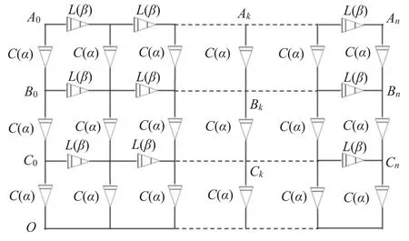
Figure 1. The FO 3 × n Fan circuit network model;fractional inductive elements ZL(ω,β),are arranged on the horizontal axis,and fractional capacitor elements ZC(ω,α) are arranged on the vertical axis.

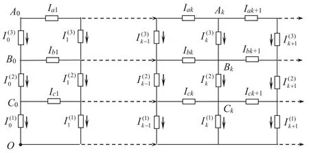
Figure 2. The topology of the FO 3×n Fan network and its parameter assumption simplified circuit model with the direction of the current parameters.

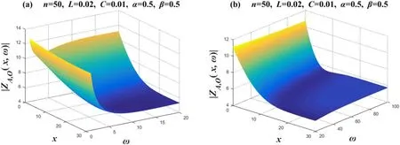
Figure 3. Set n=50 and α=β=0.5.Two 3D amplitude-frequency characteristic curves of the equivalent complex impedance ZA,O(x,ω),where figures (a) and (b) are two segmented function images,respectively.

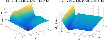
Figure 4. Set n=50,α=0.5andβ=1.Two 3D amplitude-frequency characteristic curves of the equivalent complex impedance ZA,O(x,ω),where figures (a) and (b) are two segmented function images,respectively.

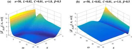
Figure 5. Set n=50,α=1 and β=0.5.Two 3D amplitude-frequency characteristic curves of the equivalent complex impedance ZA,O(x,ω),where figures (a) and (b) are two segmented function images,respectively.

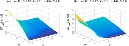
Figure 6. Set n=50,α=0 and β=1.Two 3D amplitude-frequency characteristic curves of the equivalent complex impedance ZA,O(x,ω),where figures (a) and (b) are two segmented function images,respectively.

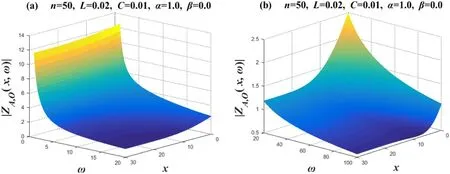
Figure 7. Set n=50,α=1 and β=0.Two 3D amplitude-frequency characteristic curves of the equivalent complex impedance ZA,O(x,ω),where figures (a) and (b) are two segmented function images,respectively.

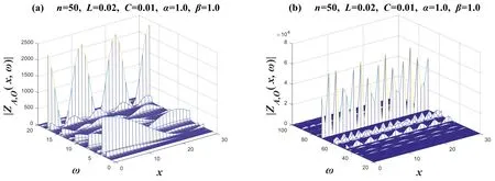
Figure 8. Set n=50 and α=β=1.Two 3D amplitude-frequency characteristic curves of the equivalent complex impedance ZA,O(x,ω),where figures (a) and (b) are two segmented function images,respectively.

Figure 9. Set n=50,α=β=0.5.Two 3D phase-frequency characteristic curves of the equivalent complex impedance ZA,O(x,ω),where figures (a) and (b) are two segmented function images,respectively.

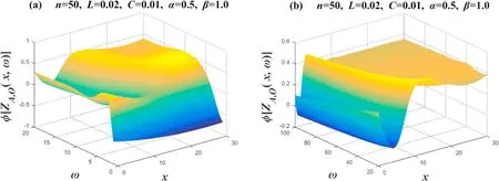
Figure 10. Set n=50,α=0.5 and β=1.0.Two 3D phase-frequency characteristic curves of the equivalent complex impedance ZA,O(x,ω),where figures (a) and (b) are two segmented function images,respectively.

Case 3.Images of phase-frequency characteristics when α=1.0,β=0.5

Figure 11 takes the values ofn=50,L=0.02,C=0.01,α=1 andβ=0.5.Image 11 and Image 10 seem to have some similarities,but their spirit is different.When you compare their vertical coordinates,you will find that the vertical coordinates of figure 10(a) are -1.0～1.0,while the vertical coordinates of figure 11(a)are-2.0～0.0;the vertical coordinates of figure 10(b) are -0.2～0.6,while the vertical coordinates of figure 11(b)are-1.0～-0.2.Specifically,their images seem to have a translational relationship.

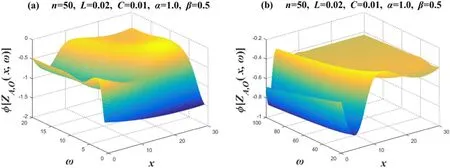
Figure 11. Set n=50,α=1 and β=0.5.Two 3D phase-frequency characteristic curves of the equivalent complex impedance ZA,O(x,ω),where figures (a) and (b) are two segmented function images,respectively.

Case 4.Images of phase-frequency characteristics when α=0,β=1.0

Whenα=0.0,β=1.0,equation (2) degenerates toZL=jωL,ZC=1/C.This is equivalent toZL=jω Lbeing a pure inductor andZC=1/C=Rbeing equivalent to a pure resistor.Image 12 and Image 9 seem to have some similarities,but their spirit is different.When you compare their vertical coordinates,you will find that the vertical coordinates of figure 9(a)are-0.8～0.0,while the vertical coordinates of figure 12(a) are 0.0～0.8;the vertical coordinates of figure 9(b) are -0.25～0.05,while the vertical coordinates of figure 12(b) are 0.5～0.8.Specifically,their images seem to have a translational relationship relative to the vertical axis.

Case 5.Images of phase-frequency characteristics when α=1,β=0

Whenα=0.0,β=1.0,then equation (2) degenerates toZL=j ωL,ZC=1/C.This is equivalent toZL=j ωLbeing a pure inductor andZC=1/C=Rbeing equivalent to a pure resistor.Image 13 and Image 12 seem to have some similarities,but their spirit is different.When you compare their vertical coordinates,you will find that the vertical coordinates of figure 12(a) are 0.0 ～0.8,while the vertical coordinates of figure 13(a) are -1.6 ～-0.8;the vertical coordinates of figure 12(b) are 0.5 ～0.8,while the vertical coordinates of figure 13(b) are -1.05 ～-0.75.Specifically,their images seem to have a translational relationship relative to the vertical axis.

Case 6.Images of phase-frequency characteristics when α=β=1.0

Figure 14 takes the values ofn=50,L=0.02,C=0.01,α=β=1.0,giving four 2D phase-frequency characteristic curves of the equivalent complex impedanceZA O(x,ω),where x={0,3,6,10} represents the complex impedance at four positions.

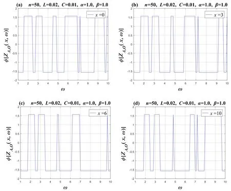
Figure 14. Set n=50,α=1 andβ=1.Four 2D phase-frequency characteristic curves of the equivalent complex impedance ZA,O(x,ω),where figures (a),(b),(c),and (d) show the phase-frequency function images of the four node positions x={0,3,6,10},respectively.

The phaseφ[ZAO(x,ω)]follows a series of jumping states with the change in frequency,as if it is an irregular pulse.We can clearly see its changing characteristics from the four images.We can seeφ?[-π/2,π/2],which is an irregular change.

5.Conclusion and comment

This article derives three general impedance formulae of the FO 3 ×nFan network model.We analyze the influence of some variables on the amplitude-frequency and phase-frequency characteristics in three different cases.At the same time,via the analysis of the FOC 3 ×nFan network,new impedance and phase results are derived.In addition,we use Matlab to draw a graphical model to describe the influence of several variables on amplitude-frequency and phase-frequency characteristics.From the series images of the amplitude-frequency and phase-frequency characteristics,problems under various conditions are considered and studied,such asRCαcircuits,RLβcircuits,LβCαcircuits andLCcircuits.

People have found that actualLCcircuits are usually FO[8–15,25–37];therefore the study of FOCs has practical application value.In this article,our results make some theoretical contributions to the development of FO 3×nFan circuit networks.

Acknowledgments

This work is supported by the National Training Programs of Innovation and Entrepreneurship for Undergraduates (Grant No.202210304006Z).

Declaration of competing interest

The authors declare that they have no known competing financial interests or personal relationships that could have appeared to influence the work reported in this paper.

ORCID iDs