Effects of connected automated vehicle on stability and energy consumption of heterogeneous traffic flow system
2024-03-25 09:30:10JinShen申瑾JianDongZhao趙建東HuaQingLiu劉華清RuiJiang姜銳andZhiXinYu余智鑫
Chinese Physics B 2024年3期
Jin Shen(申瑾), Jian-Dong Zhao(趙建東),2,?, Hua-Qing Liu(劉華清),Rui Jiang(姜銳), and Zhi-Xin Yu(余智鑫)
1School of Systems Science,Beijing Jiaotong University,Beijing 100044,China
2Key Laboratory of Transport Industry of Big Data Application Technologies for Comprehensive Transport,Beijing Jiaotong University,Beijing 100044,China
3School of Maritime and Transportation,Ningbo University,Ningbo 315000,China
Keywords: heterogeneous traffic flow,CAV,linear stability,nonlinear stability,energy consumption
1.Introduction
With the promulgation of national policies advocating the promotion of intelligent vehicles, connected automated vehicle (CAV) is increasingly widespread and popular.The CAV has considerable potential to enhance traffic efficiency, however, the full marketing of CAV requires a process and the heterogeneous traffic flow consisting of HDV and CAV will exist for a long time, so it is of great theoretical and practical significance to study the stability and energy consumption of the heterogeneous traffic flow under varying levels of CAV permeability.
In the realm of traffic flow models, the construction of an appropriate model serves as a potent approach to investigating the characteristics of traffic flow.Traffic flow models are typically classified as three categories: micro model,meso model, and macro model.Microscopic model focuses on individual vehicle behavior, while macroscopic model captures overall traffic flow behavior.Newell[1]proposed an optimization function for headway distance that governs speed adjustments in following vehicles.Bandoet al.[2]introduced an optimal velocity model,which accurately simulates various characteristics of real-world traffic flow.Jianget al.[3]put forth a full velocity difference model to establish conditions for traffic flow stability.Lighehill and Whitham[4,5]presented a macroscopic model of traffic flow,known as the Lighthill-Whitham-Richards (LWR) model, which characterizes the continuous medium features of traffic motion.Payne[6]incorporated dynamical equations into the continuum model to create a new traffic dynamics model that combines both continuum and dynamical equations.Jinet al.[7-10]proposed a method to convert a microscopic model into a macroscopic one,resulting in a macroscopic traffic flow model that describes the road environment.
In the aspect of traffic flow capacity, the emergence of CAV offers the possibility of solving traffic problems at root.Zonget al.[11]investigated the CAV homogeneous flow under different mixing scenarios through simulation, the results showed that the proportion of CAV is higher,the time for the platoon as a whole to recover to a smooth state is shorter,and the traffic efficiency is improved.Talebpouret al.[12]conducted experiments on a four-lane roadway in Chicago for the traffic flow operation problem of CAV reserved lanes,and the simulation results showed that CAV reserved lanes are beneficial to capacity improvement when the CAV market rate reaches 30%to 50%.Ye and Yamamoto[13]developed a specialized CAV lane traffic flow model, and the simulation results showed that the CAV lane can be fully utilized only in medium density traffic condition.
In the area of stability analysis for heterogeneous traffic flow,Qinet al.[14,15]studied the stability of heterogeneous traffic flows and verified the correctness of the analytical results through numerical simulation experiments.Luoet al.[16]analyzed the linear stability conditions of heterogeneous traffic flow by using the characteristic equation method,and demonstrated that the CAV can enhance the linear internal stability of heterogeneous traffic flow.Zhanget al.[17]established a hybrid car following model for adaptive cruise vehicle and normal vehicle,analyzed the linear and nonlinear stability of the heterogeneous traffic flow.
In respect of energy consumption, Penget al.[18]proposed a new lattice hydrodynamic model to calculate the energy consumption of the traffic system,and the results showed that by considering delay control under the V2X environment,energy consumption can be reduced.Guoet al.[19]presented a two-line traffic system, and the results showed that the energy consumption can be reduced by considering delayed flow control information.Zenget al.[20]simulated the influence of CAV and platoons on traffic flow and energy consumption,and the results showed that increasing the proportion of CAV can effectively reduce the average energy consumption.
Although it is believed that the CAV has widespread application prospects,[21,22]their practical effectiveness and influence on heterogeneous traffic with varying permeability of CAV in relation to conventional human driven vehicles remain uncertain.[23-25]To shed light on the influences of CAV on heterogeneous traffic, in this work a systematic and targeted study is carried out.
In this work, we first develop a novel heterogeneous car following model by optimizing speed and headway terms,which combines both HDV and CAV.Subsequently,we transform the microscopic model into a macroscopic representation, yielding a continuum macroscopic dynamical heterogeneous traffic model.We then conduct comprehensive linear and nonlinear stability analyses of the heterogeneous traffic flow, culminating in the derivation of the density wave solution of the KdV-Burgers equation.By employing this method,we elucidate the characteristics and stability of the traffic system.Finally,we perform simulations to thoroughly investigate the influence of varying CAV permeability on the stability and energy consumption of the traffic system.
2.Heterogeneous traffic model
The full velocity difference (FVD) model proposed by Jianget al.[3]addresses the issue of traffic congestion arising from the headway between two vehicles being less than the safety distance and the rear speed being too fast.Sunet al.[26]took the backward-looking effect into account in the FVD and constructed a car-following model as follows:
Using this model as the following model for HDV and considering that the CAV is able to integrate modern communication and network technologies through on-board sensors, the interconnection of distance and speed between vehicles can be realize,and the following model of CAV is proposed:
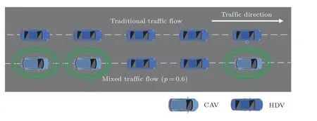
Fig.1.Comparison among traffic systems.
With the gradual development and recognition of CAV,the mixing of CAV and HDV will be seen everywhere.Assuming that HDV and CAV are evenly and randomly distributed on the road as depicted in Fig.1,the microscopic heterogeneous traffic flow car-following model can be articulated through the following equation:

Table 1.Summary of symbols involved in this paper.
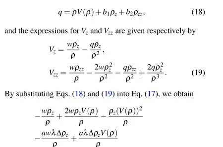
We can know the following expressions[30]
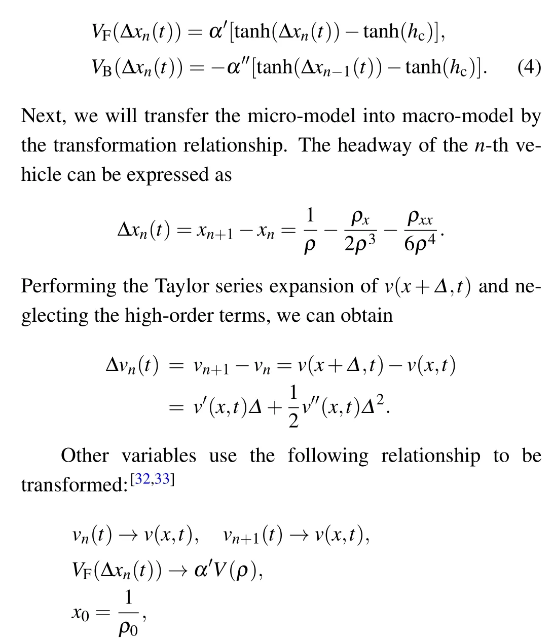
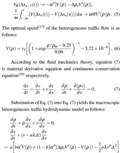
which contains the continuity equation and the hydrodynamic equation of the heterogeneous traffic flow respectively.
3.Linear stability analysis of heterogeneous traffic flow
In order to analyze the various properties of the macroscopic heterogeneous traffic hydrodynamic model, the linear stability method is used.Linear stability analysis of traffic flows is a prerequisite for nonlinear analysis and is the basis for distinguishing between stability zones.
Assuming that the equilibrium traffic flow is the initial state of the heterogeneous traffic system, the speed (v0) and the density (ρ0) of the heterogeneous traffic flow will remain consistent in this state.Then a minor perturbation to the heterogeneous traffic flow can be denoted as
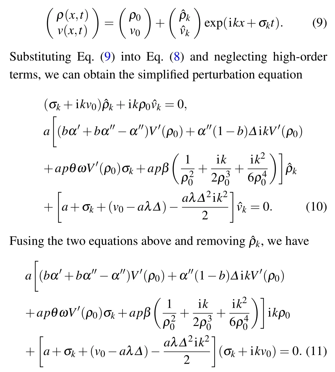
Conducting the series expansion ofσkasσk= (ik)σ1+(ik)2σ2+···, neglecting higher order terms, and taking only the first item and the second items,and substituting them into Eq.(12),equation(12)is simplified into

Whenσ2is negative,the initial uniform steady flow state becomes unstable;whenσ2is positive,the steady flow state is stable,therefore we can obtain the stability conditions
Mapping traffic flow system stability regions are based on stability conditions.Traffic system stabilities differ when heterogeneous traffic flows have different permeability of CAV.From Fig.2(a), it can be shown that the stable area is above the curve and the unstable area is below the curve.The area above the curve gradually expands as the permeabilitypof the CAV increases and the stability of the system gains strength.This means that increasing the proportion of CAV in heterogeneous traffic flows can effectively improve the stability of the traffic system.

Fig.2.(a)Stable area and unstable area,and(b)neutral stability curves for different permeability p.
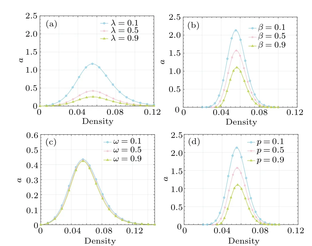
Fig.3.Comparison of regions of stability and stability curves among different models.
Figure 3 presents a comparison of the regions of stability among different models.Figure 3(a)shows the changes in the stability curve of the FVD model with parameterλ.Figure 3(b)shows the model built by adding the optimization term of headway to the FVD model,the stability curve changes with coefficient of the distance optimization termβ, and it is observed that an increase inβresults in a larger region of stability.Figure 3(c) exhibits the model crafted by integrating the speed optimization term into the FVD model.As the coefficients of the memory velocity optimization termωfluctuates,the stability curve changes.Notably,an escalation inωengenders an expanded realm of stability.Figure 3(d) exhibits the curve of stability varying as the permeabilitypof CAV fluctuates within the heterogeneous traffic flow model put forth in this work.By carefully observing Figs.3(b) and 3(c), it can be deduced that the two additional terms introduced into our model have a positive effect on improving the stability of heterogeneous traffic flow through considering the characteristics of CAV.From Figs.3(a)and 3(d), it can be observed that the heterogeneous traffic flow model constructed in our study has a larger region of stability and stronger stability than the FVD model,indicating its practical significance.
4.Nonlinear stability analysis of heterogeneous traffic flow
This section will perform the nonlinear analysis of the heterogeneous traffic system to study the behavior of the system around the neutral stability curves.We start with introducing a new coordinate system.The conversion of the new coordinate system[34]takes the following form:

In the traffic flow theory,flowqis equal to the product of density and speed,i.e.,q=ρ·v.[35]
A Taylor expansion of flowqprovides Eq.(18),with only the first term and the second-order term retained,
The parametersb1andb2are to be determined through the coefficients of the variableρzandρzz.When the values of the coefficients are zero, an expression forbcan be obtained as follows:
whereξis determined by the initial state and is an arbitrary constant.
5.Simulation and analysis
Now we will study the influence of permeability and energy consumption on heterogeneous traffic system from the simulations perspective.When small perturbation is injected into the equilibrium stream,the magnitude of the fluctuations in the perturbation amplifies or disappears completely over time.The latter will correspondingly enter into a steady state.
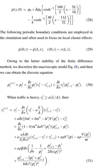
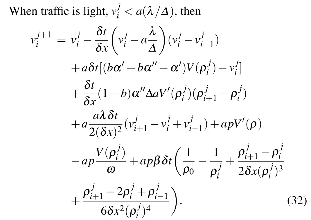
In this section the spatiotemporal evolution of heterogeneous traffic behaviour with density and velocity will be analyzed.Here, the research focuses on cluster effect and the stability for different initial densities and permeabilitypin the development of heterogeneous traffic.Simulation related parameters are listed as follows:δρ= 0.01,δx= 100 m,δt=1 s,L=32000 m,andVf=30 m/s,whereδρis a minor disturbance to the steady density;δρis the time step;δxis the space step of the simulation;Lis the length of the road.The initial density of the road is given as follows:[38]
5.1.Verification
The stability of the heterogeneous traffic system will be verified in order to verify the above theoretical analysis.We choose two points 1 and 2 as follows: point 1 is selected in the stable zone and point 2 is selected in the unstable zone.As we can see in Fig.4, the densityρis 0.02 and the sensitivity coefficientais 0.4 at point 1,while at point 2 the densityρis 0.06 and the sensitivity coefficientais 0.2.Given a perturbationδρ=0.01,the simulation is performed for two different scenarios.

Fig.4.Selection of validation points.
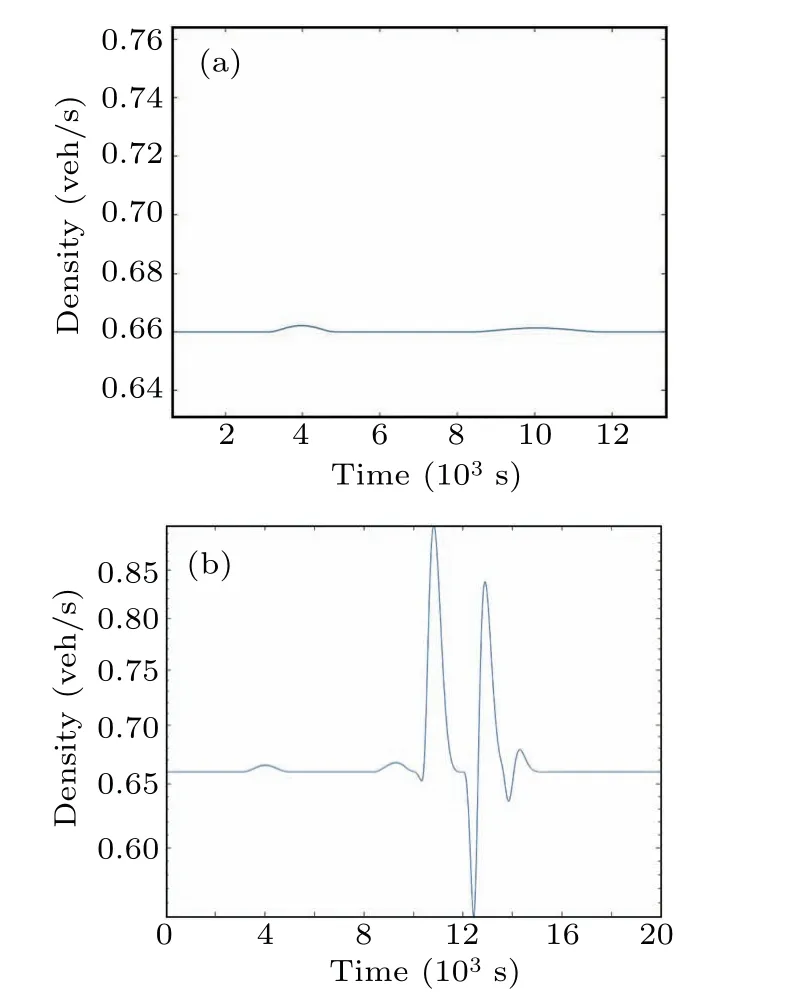
Fig.5.Evolution of disturbance in two scenarios.
Figure 5 shows the simulations results of the heterogeneous traffic flow.Figures 5(a) and 5(b) present the curves of traffic density varying with time under a small disturbance to the traffic flow at point 1 and point 2 respectively.When the traffic flow is disturbed at the stable point 1, the traffic is affected slightly but quickly restores stability, resulting in no jamming; when the traffic flow is disturbed at the unstable point 2,the traffic density is oscillatory and the traffic flow appears to stop and go,resulting in congested road.
5.2.Local effect
Figure 6 shows the spatial and temporal evolution of the density of heterogeneous traffic flows.From a spatiotemporal viewpoint,whenp=0.1,it becomes apparent that a slight perturbation imparted to the heterogeneous traffic flow triggers off a fluctuation that gradually diminishes in magnitude as it traverses through the temporal domain and spatial domain.Remarkably,the perturbation propagates from the downstream section to the upstream section of the road, culminating in a comprehensive instability within the traffic flow.As the permeability of CAV continues to increase, the perturbation is still amplified as it propagates towards the upstream of the road,leading to instability of the traffic flow.However,when the permeability increases to a certain level, as indicated in Fig.6(d), the perturbation is not infinitely amplified but suppressed during propagation,and finally the traffic flow settles down,the traffic flowbecoming steady at this moment.Therefore, the higher permeability of intelligent autonomous vehicle can effectively reduce the instability of the traffic flow and eventually make the heterogeneous traffic flow stable, which is consistent with the stability analysis results in the previous part.
Under periodic boundary conditions, we find that congestion of the downstream affecting the upstream of the road.As the permeabilitypgrows,the road swarms with more and more CAVs, the congestion propagation is suppressed, indicating that the congestion area is diminishing.Meanwhile,the simulation reveals the go-and-stop phenomena with varying densities during the evolution of traffic flow.
Various initial densities can also have significant influences on the traffic flow evolution.Figure 7 shows different traffic flow patterns under different initial densities forp=0.5.Whenρ0=0.028 veh/m, traffic flow remains relatively stable in low density area.With the initial density increasing,as shown in Figs.7(b)and 7(c),the small disturbance given to the road causes the flow to suffer a loss of stability and accumulate congestion, the road has go-and-stop waves.In addition, the occurrence of local clustering can be seen in Fig.7(b),where two congestions become one congestion.The local clustering phenomenon is more likely to happen while the traffic congestion is more severe.Eventually, the traffic flow returns to the steady state in Fig.7(d).
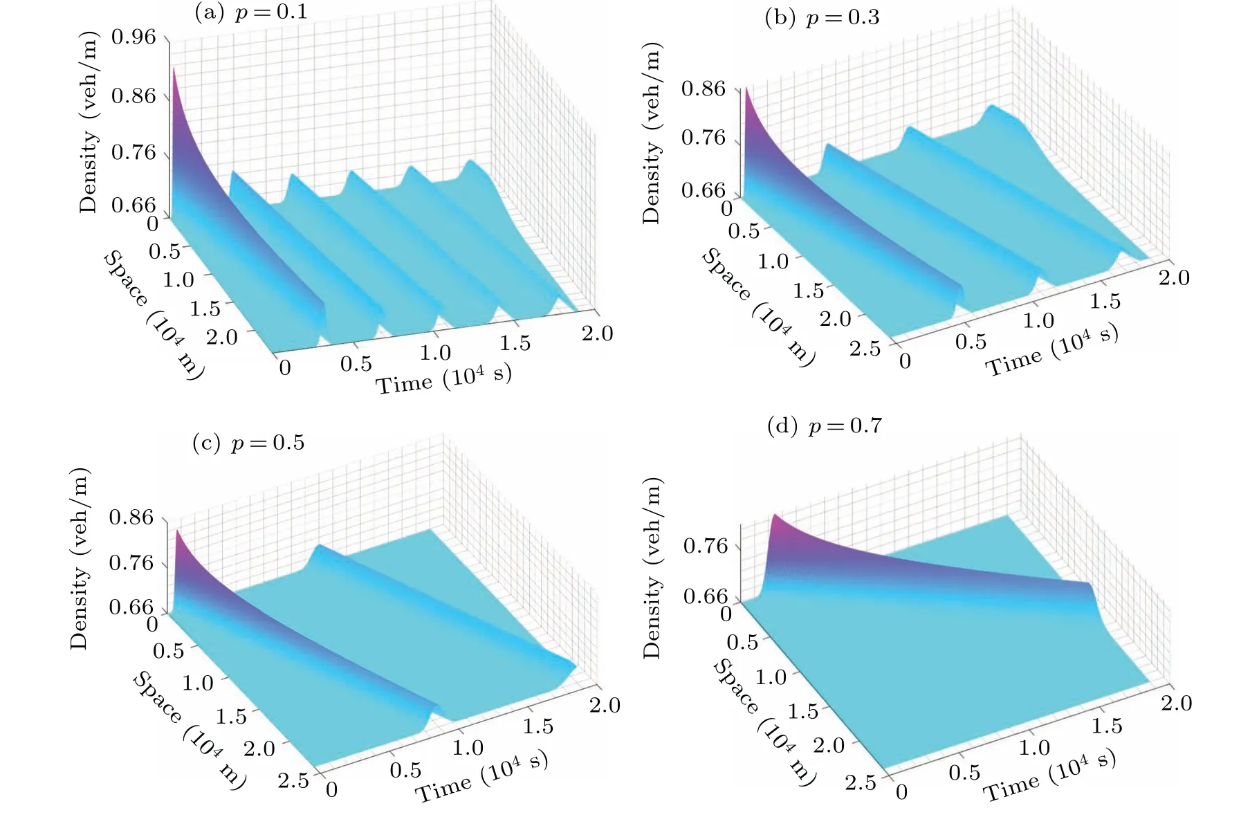
Fig.6.Spatiotemporal evolution of heterogeneous traffic with different values of penetration p of CAV.
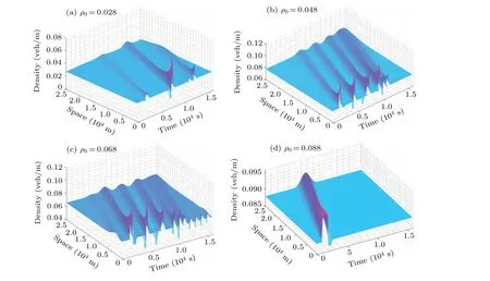
Fig.7.Spatiotemporal evolution of heterogeneous traffic with initial density ρ0.
5.3.Energy consumption
In order to analyze the energy consumption of the heterogeneous traffic flow, an energy consumption formula is given based on the principle of kinetic energy[20]as follows:
Equation (33) represents the corresponding energy emission under the condition of(i,j).Thus the overall energy consumption of the traffic system is
The total energy consumption(TEC)of the system is defined as the energy consumption during the simulation, including the simulation time,which is expressed as

Fig.8.Spatiotemporal evolutions of energy consumption with permeability.
According to the effects of different initial densities on traffic flow evolution analyzed in Fig.7, the initial density of the simulation is set to 0.068 in this subsection.Figure 8 shows the spatial pattern and temporal pattern of energy consumption at different CAV permeability,where the green indicates lower energy consumption and red represents higher energy consumption,and the trend of color changing from green to yellow to red indicates higher and higher levels of energy consumption.In Fig.8(a), it can be clearly observed that the red area is larger and more obvious than in Fig.8(b), which indicates that the system energy consumption is higher when the proportion of CAV on the road is lower.Correspondingly,as the proportion of CAV increases, the energy consumption peaks in Figs.8(c)and 8(d)gradually decrease until the energy consumption fluctuations gradually disappear and the state of the traffic system becomes more and more stable.
Figure 9 exhibits more clearly the energy consumption at 15000 m of the road corresponding to the results of Fig.8.In Fig.9(a), the number of CAVs is low and the peak of the energy consumption curve is higher than in Figs.9(b) and 9(c)and the area of the colored area is larger.As CAV increases,the top of the energy consumption curve decreases from about 0.2 to 0.15 and the region of the painted area decreases significantly.It indicates that the energy consumption level of the heterogeneous traffic system can be reduced by increasing the road CAV permeability.
Meanwhile, we calculate the energy consumption of the traffic system and TEC during the simulation in Fig.10, the simulation conditions are the same as those used previously.This can be seen in Fig.10(a),where the CAV permeability is lower at 0.1,the green area is wider and the energy consumption of the transportation system is higher at 22356.53.As the CAV permeability increases to 0.3, the number of CAVs on the road rises and the total energy consumption falls from 22356.53 to 18667.70, namely by 16.50%.Then the permeability continues to increase to 0.5 and the TEC decreases from 18667.70 to 14560.81,i.e.,by 22.00%.When the permeability increases to 0.7, the total energy consumption eventually decreases to 10576.97, which is consistent with the trend of traffic flow stability.It indicates that the smaller the energy consumption of the traffic system,the more stable the level of the corresponding traffic flow is.The trends of both energy consumption and stability verify the effectiveness of introducing CAV.

Fig.9.Profiles of energy consumption of j=1.5×10⁴ for permeabilities p=0.1(a),0.3(b),0.5(c),and 0.7(d).
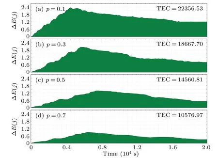
Fig.10.Variations of energy consumption with time for j=1.5×10⁴ and permeability p=0.1(a),0.3(b),0.5(c),and 0.7(d).
6.Conclusions
In this work, we put forth a continuum heterogeneous traffic flow model for HDV and CAV approaching the actual road conditions.This model takes into consideration the intricate interplay of information exchange among CAVs, including optimizing the perception of speed and distance with respect to preceding and subsequent vehicles.Subsequently,we derive the linear stability condition of the model by introducing a small perturbation into the equilibrium system, and conduct a thorough analysis of linear stability and nonlinear stability.Finally, we employ numerical simulation based on the macroscopic heterogeneous traffic flow model to investigate the effect of CAV permeability on the stability and energy consumption of the system, and the ensuing traffic phenomena.The experimental findings reveal the following points.
(i) With the ascendancy of CAV permeability, the fluctuation of heterogeneous traffic flow density becomes smaller and smaller, leading to an augmented stability of the traffic system.The integration of CAV effectively curtails the propagation of traffic congestion, enhancing the resilience of the heterogeneous traffic flow against disturbances.
(ii)Distinct initial densities of traffic system,even under equivalent CAV permeability, wield a pronounced influence on the stability of traffic flow.Higher initial density exacerbates the likelihood of traffic congestion, which triggers off local clustering effect that undermines the smoothness of traffic flow.This phenomenon manifests as a stop-and-go pattern,where vehicular movement experiences intermittent halts and restarts, further compromising the stability of the traffic system.
(iii) The total energy consumption of the heterogeneous traffic system decreases as the CAV permeability rises.As the permeability of CAV gradually rises from 0.1 to 0.7,with each successive augmentation of 0.2,the total energy consumption of the system undergoes a noteworthy diminution of 16.5%,22%,and 27.36%respectively.
Acknowledgements
Project supported by the Fundamental Research Funds for Central Universities, China (Grant No.2022YJS065) and the National Natural Science Foundation of China (Grant Nos.72288101 and 72371019).

- Chinese Physics B的其它文章
- A multilayer network diffusion-based model for reviewer recommendation
- Speed limit effect during lane change in a two-lane lattice model under V2X environment
- Dynamics of information diffusion and disease transmission in time-varying multiplex networks with asymmetric activity levels
- Modeling the performance of perovskite solar cells with inserting porous insulating alumina nanoplates
- Logical stochastic resonance in a cross-bifurcation non-smooth system
- Experimental investigation of omnidirectional multiphysics bilayer invisibility cloak with anisotropic geometry