Sharing quantum nonlocality in the noisy scenario

Shu-Yuan Yang(楊舒媛), Jin-Chuan Hou(侯晉川), and Kan He(賀衎)

College of Mathematics,Taiyuan University of Technology,Taiyuan 030024,China

Keywords: Bell nonlocality,quantum measurement,quantum noise

1.Introduction

Quantum nonlocality is a kind of quantum resource distinct from entanglement and Einstein–Podolsky–Rosen(EPR) steering, and has broad applications in quantum information processing.[1–4]Nonlocal correlations offer a quantum advantage in communication complexity problems,[5]device-independent quantum cryptography,[6,7]randomness expansion,[8]and measurement-based quantum computation.[9,10]Quantum nonlocality can be demonstrated by violation of Bell inequalities (or Bell-type inequalities).[11–13]Furthermore, researchers have also developed various experimental techniques on quantum nonlocality.[14–17]

In previous researches,scientists explored the limitations of nonlocality by asking whether a pair of entangled qubits could produce a long sequence of nonlocal correlations in Refs.[18–21].Silvaet al.first introduced this sequential scenario (see Fig.1) and demonstrated that at most two sequential observers (Bobs) could share nonlocality with a single Alice through weak measurements.[18]Since then, additional theoretical and experimental findings on nonlocality sharing have been obtained.[22–31]Brown and Colbeck found a measurement strategy such that there exists an unbounded number of independent Bobs who are able to violate the Clauser–Horne–Shimony–Holt (CHSH) inequality with a single Alice by sequentially measuring one half of a maximally entangled pure two-qubit stateρAB(1)=|φ+〉〈φ+| with.[27]Folettoet al.implemented experimentally the nonlocality-sharing strategy.[32]Zhang and Fei extended the aforementioned results to the case of arbitrary finite-dimensional systems.[33]In Refs.[34,35], problems on sharing network nonlocality were also discussed.However,the above discussions are always limited to the ideal scenario,where the initial states and measurements are noiseless.

Recently the topics of noisy network nonlocality were focused on in Refs.[36,37].Mukherjee studied error tolerance of nontrilocal correlations in noisy triangle networks,[36]where different sources of imperfections were considered, such as errors in entanglement generation, communications over noisy quantum channels and noises in measurements.[38–40]Furthermore,the similar problem on persistency of the non-n-local correlations in noisy linear networks was analyzed in Ref.[37].The aforementioned researchers discovered that the influence of noises can result in the decay of nonlocality in quantum networks.So can it in the nonlocality-sharing scenario.In this paper,we analyze persistency of sharing nonlocality in the noisy scenario, where the initial states and measurements have errors in entanglement generation and white noises,respectively.

The study presents the conditions for nonlocality sharing termination and infinite nonlocality sharing,respectively,and uses images to reflect the impact of noise on the maximum number of independent Bobs who can share the nonlocality of the noisy initial state with the single Alice.Furthermore, we investigate the noisy nonlocality sharing in high-dimensional bipartite systems.

The paper is arranged as follows.In Section 2,we review some basic results on sharing nonlocality.In Section 3, we first focus on the case that the initial state is the two-qubit one.Here,noises from entanglement generation and measurements are introduced.Furthermore, we obtain two sufficient conditions of the persistency of sharing nonlocality noisily, and analyze the change patterns of the maximal number of Bobs who can share nonlocality with Alice under the influence of different noises.In Section 4, we devote to generalizing the persistency to arbitrary finite-dimensional systems.

2.Preliminaries

In this section, we review the results on the nonlocalitysharing scenario(see Fig.1).

2.1.Detection of nonlocality

The quantum nonlocality of a bipartite stateρABcan be proved by violating Clauser–Horne–Shimony–Holt (CHSH)Bell inequality[41]

where〈AxBy〉=∑a,b(?1)a+bp(a,b|x,y) is the joint expectation value of the observations of Alice and Bob when their settings arexandy(x,y ∈{0,1}),and binary outcomes areaandb(a,b ∈{0,1}), respectively.AiandBiare observables withr(Ai)≤1 andr(Bi)≤1,i=0,1.Denote byr(A) the spectral radius of the matrixA.The distributions are given by the Born rule

where ∑a(?1)aAa|x=Axand ∑b(?1)bBb|y=Byfor Alice’s measurement set{Aa|x}a,xand Bob’s one{Bb|y}b,y.

2.2.The sequential nonlocality-sharing scenario

LetHAandHBbe finite-dimensional complex Hilbert spaces andρAB(1)a bipartite state acting onHA ?HBwith dim(HA)=sand dim(HB)=t.Denote byImthem×midentity matrix.In Ref.[18], the sequential nonlocality-sharing scenario was proposed(see Fig.1).Here Alice and Bob(1)share an initial entangled bipartite stateρAB(1).Suppose Bob(1)performs the measurement according to binary inputY(1)=ywith binary outcomeB(1)=b, the postmeasurement state shared between Alice and Bob(2)can be described by the Lüders rule,[27]i.e.,

whereBis the positive operator-valued measurement(POVM) corresponding to outcomebof Bob(1)’s measurement for inputy.Repeating this process,the stateρAB(k)shared by Alice and Bob(k)can be computed as

whereBis the POVM corresponding to outcomesbof Bob(k?1)’s measurements for inputy.

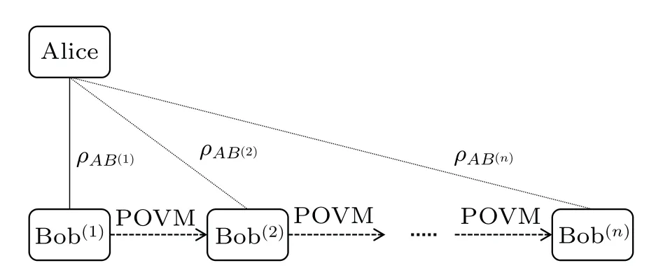
Fig.1.A bipartite entangled state ρAB(1) is initially shared between Alice and Bob(1).Bob(1) performs a POVM on his part.Denote by ρAB(2)the post-measurement state.Bob(2) also performs a POVM, and this process continues until Bob(n).One want to ask how many Bobs can share the nonlocality with Alice at most.

whereσj(j= 1,2,3) are Pauli matrices,θ ∈(0,π/4] andηk ∈(0,1)for anyk=1,2,...,n.

forθ ∈(0,π/4]andηk ∈(0,1),k=1,2,...,n.When bothsandtare odd,a set of POVMs can be given by

forθ ∈(0,π/4]andηk ∈(0,1),k=1,2,...,n.

3.Sharing nonlocality in noisy two-qubit systems

In this section, we study persistency and termination on sharing nonlocality noisily with initial two-qubit states.

Before that,we first introduce the noise generation.

3.1.Noise generation

The first kind of noises comes from entanglement generation of the initial state.In the experiment,a two-qubit entangled stateis generated by the action of the Hadamard gateHand CNOT gate onζ=|10〉〈10|.

Letαandδdenote the noisy parameters characterizing theHgate and CNOT gate, respectively.Starting fromζ=|10〉〈10|,and the noisy Hadamard gate generates[38]

Subjection ofζ'1to noisy CNOT gives

Denote byT(ρ)=(wi,j)3×3the correlation matrix whose entries are given bywi,j= tr[ρ(σi ?σj)].ThenT(ˉρAB(1)) =diag(?αδ,αδ,δ).

Secondly, the white noises are fixed on POVMs{A0|i,A1|i}i=0,1andof parties Alice and Bob(k),k=1,2,...,n.Letβ1∈[0,1] characterize the noisy measurement set{A0|0,A1|0}in the sense that it fails to detect with probability 1?β1,i.e.,β1parametrizes a faulty measurement device.Similarly,the noisy parameters for measurements{A0|1,A1|1},andare denoted byβ2,γkandμk,k=1,2,...,n, respectively, andβ2∈[0,1],γk ∈[0,1],μk ∈[0,1].If dim(HA)=sand dim(HB)=t,then noisy POVMs can be represented as

We takes=t=2 when we consider the case of the initial state being a two-qubit state.Then the corresponding noisy observables are

Combing Eqs.(5)–(8) with the form of noisy POVMs (see Eqs.(19)–(22)), when the initial sharing state is a two-qubit state we write the noisy measurement strategy as follows:

3.2.Persistency of the noisy nonlocality-sharing scenario

In order to analyze the persistency, we first calculate the expected CHSH valuewith the noisy initial state and noisy POVMs.The detail of the proofs for our theorems will be presented in the appendix.

Theorem 1 For the noisy initial state ˉρAB(1)in Eq.(18),if Alice and Bobs perform noisy measurements in Eqs.(27)–(30)and Eqs.(31)–(32),respectively,then the expected CHSH value ofρAB(k)is given by

whereθ ∈(0,π/4],δ,α,βi,ηk,γkandμk ∈[0,1]fori=1,2,k=1,2,...,n.

In the following,we provide two sufficient conditions of persistency of sharing nonlocality noisily.

Theorem 2 For the noisy initial state ˉρAB(1)in Eq.(18),assume Alice and Bobs perform noisy measurements in Eqs.(27)–(30)and Eqs.(31)–(32),respectively,then there existnBobs sharing the nonlocality of ˉρAB(1)with the single Alice if there existsε ＞0 such that

where

with

Theorem 3 For the noisy initial state ˉρAB(1)in Eq.(18),assume Alice and Bobs perform noisy measurements in Eqs.(27)–(30) and Eqs.(31)–(32), respectively, ifγn(β1+β2)δ= 2, then there existnBobs who can share the nonlocality of the noisy initial state ˉρAB(1)with the single Alice for arbitrary given noisy parametersα,γk,μj ∈(0,1],k=1,2,...,n?1 andj=1,2,...,n.

The set{α,δ,β1,β2,μk,γk}nk=1consists of all noisy parameters.The condition in Theorem 2 reveals how the persistency of sharing nonlocality in the noisy scenario depends on all noisy parameters.If, for somensuch that Eq.(34) holds for someε ＞0, but there is noε ＞0 so that Eq.(34) holds forn+1, then Alice can at most share the nonlocality withnBobs, and the sharing process stops atnth step.The persistency condition in Theorem 3 is more pragmatic and some what surprising.Note thatγn(β1+β2)δ=2 meansγn=β1=β2=δ=1,i.e.,their corresponding noises vanish.Theorem 3 reveals that, if the noises parametersβ1=β2=δ= 1 and the noise parameterγn=1 forn ≥1, then Alice can share nonlocality at least withnBobs whatever the noise parametersα,take any values in (0,1].Why the phenomenon in Theorem 3 happens? One can find from the proof of Theorem 3 that whenθis small enough, each index of persistencyηk=ηk(θ)always can lie in(0,1)for arbitrary nonzero noisy parametersα,.Recall the parameterθcomes from the Alice’s measurement.This means Alice’s appropriate measurement device can counteract the influence on persistency under noises from the Hadamard gate and Bobs’measurements.

In the aforementioned theorems,it is always assumed that the initial state is a kind of special noisy maximal entangled states.Finally, we consider the nonlocality-sharing problem on the general case that the initial state is an arbitrary twoqubit state.For an arbitrary two-qubit stateρAB(1), assume that Alice and Bobs perform noisy measurements in Eqs.(27)–(30)and Eqs.(31)–(32),respectively,it follows that the CHSH value is

whereθ ∈(0,π/4],δ,α,βi,ηk,γkandμk ∈[0,1]fori=1,2,k= 1,2,...,n.Similar to the proof of Theorem 3, we can claim that ifγn(β1+β2)p=2, then there existnBobs who can share the nonlocality of the initial stateρAB(1)with the single Alice for arbitrary given noisy parametersγk,μj ∈(0,1],k=1,2,...,n?1 andj=1,2,...,n.

3.3.Termination of sharing nonlocality in noisy scenarios

As we see from Theorems 2 and 3, different kinds of noises result in different influences on the decay of nonlocality.In this section, we discuss the question how the noises influence the persistency of sharing nonlocality.We divide the discussion to two cases: state noises and measurement noises.It is assumed that the noisy parameters are always nonzero,the given noisy initial state ˉρAB(1)is presented in Eq.(18)and the noisy measurements are presented in Eqs.(27)–(32).

3.3.1.Errors on entanglement generation

Letδ=β1=β2=μk=γk=1 for allk=1,2,...,n,we investigate the influence of the noisy parameterαon the persistency.By Theorem 1,we have in this case that

For anyε ＞0,define a sequence(ηi(θ,α,ε))irecursively asand

whenever 0＜ηk?1(θ,α,ε)＜1,whereθ ∈(0,π/4]andα ∈[0,1].One can check that 0＜ηm(θ,α,ε)＜1 for allm ≤kif and only if there existkBobs who can share nonlocality with Alice, and the nonlocality-sharing behavior terminates once if there islsuch thatηl(θ,α,ε) equals to or lager than 1.As we know from Ref.[27], ifα=1 (this means all the corresponding noise vanishes),then for any given positive integerk, there existsθclosed to 0 enough such that one can choseηj(θ,α)∈(0,1) for allj=1,2,...,k.However, by Theorem 3, the similar can be done for any noise parameterα ∈(0,1].

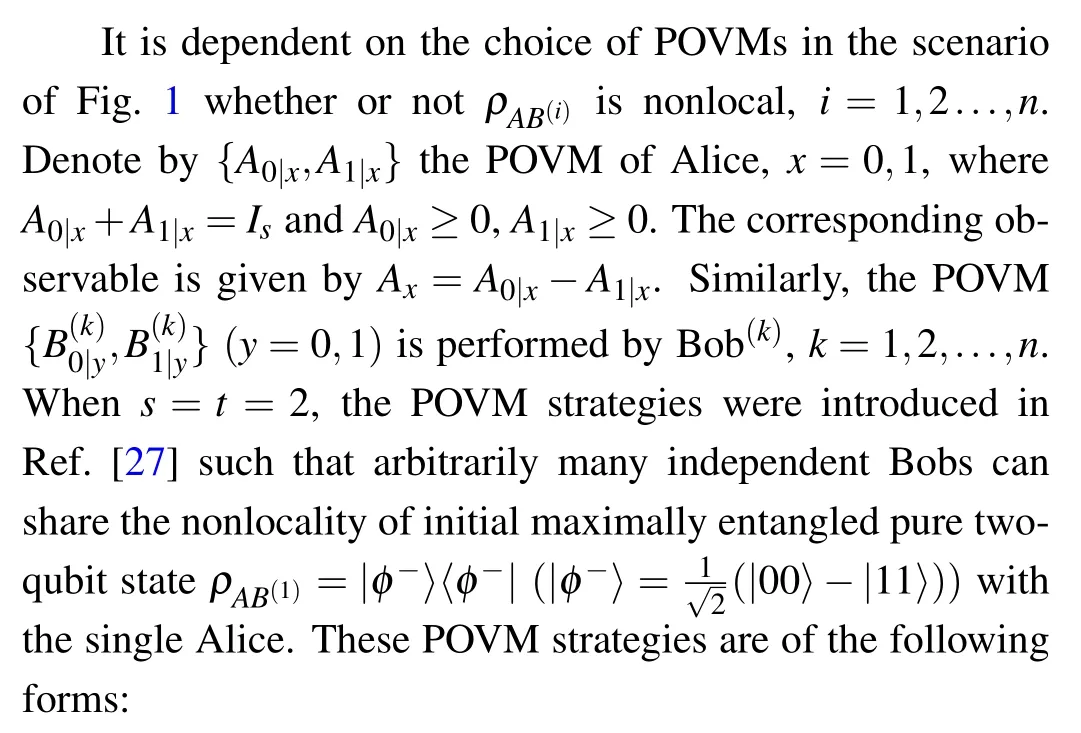
We plot the functional values ofηk(θ,α) as a function ofαin the image (see Fig.2(a)) fork=1,2,3,4 when we takeε=10?5.In Fig.2(b), the correspondingηk(θ,α)falls into the interval (0,1) when (θ,α) lies in the lower region of each curve fork= 1,2,3,4.Whenαmoves from 1 to 0 andθmoves from 0 to 1 respectively, the maximal numberof Bobs who can share the nonlocality with Alice will decrease and can be calculated by determining how manyηk(θ,α)s lie in the interval (0,1).From Fig.2(b),one can see clearly the value ofwhen (θ,α) lies in the given region [0.05,π/4]×(0,0.95].For instance, there are at most three Bobs sharing the nonlocality with Alice when(θ,α)=(0.1,0.9).

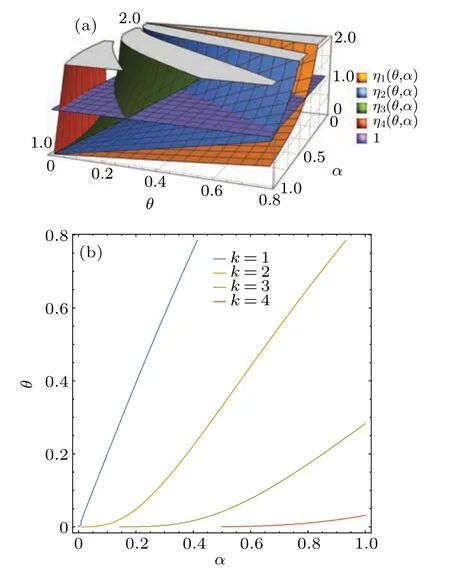
Fig.2.(a)The yellow,blue,green and red surfaces represent the values of η1(θ,α),η2(θ,α),η3(θ,α)and η4(θ,α),respectively,as functions of parameters θ and α.The purple plane denotes the unit plane.Due to the limit of accuracy of the computer calculation, the images with k ≥5 cannot be plotted.(b) The blue, orange, green and red curves represent η1(θ,α)=1,η2(θ,α)=1,η3(θ,α)=1 and η4(θ,α)=1,respectively.

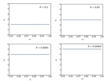
Fig.3.The value of the vertical axis n= is the maximal number of Bobs who can share nonlocality with Alice.

To see what happens when (θ,α) lies in the region(0,0.05)×(0.95,1),we exhibit the change pattern ofdependent on the noise parameterα ∈(0.95,1)whenθis fixed as 0.5,0.05,0.0005 and 0.00005 respectively(see Fig.3).It is surprising that whenθis given,the value ofkeeps invariant ifαmoves from 0.95 to 1.Also,in Fig.3,asθdecreases,theincreases,i.e.,the persistency becomes better.

Moreover,when we observe the influence of the noise parametersδandβ1+β2in Eq.(33), it is not difficult to conclude that the change pattern ofonδand that onβ1+β2are the same.Therefore,we will merge the discussions of the above two cases to Case 2 in Subsection 3.3.2 hereinafter.

3.3.2.Noises come from measurements

Case 1.For anyn ≥1, cosider the case thatγ1=γ2=··· =γk=γandα=δ=β1=β2=μk= 1 for allk=1,2,...,n.By Theorem 1 we have

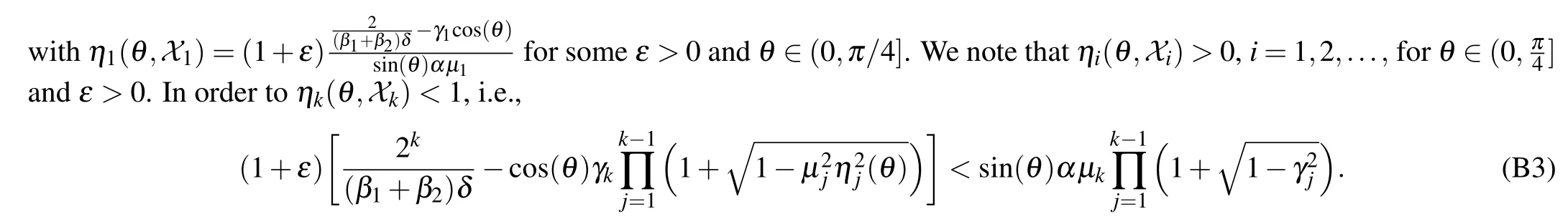
Take a smallε ＞0 and define a sequence{ηi(θ,γ,ε)}ni=1by

whenever 0＜ηk?1(θ,γ,ε)＜1 withη1(θ,γ,ε) = (1+forθ ∈(0,π/4]andγ ∈[0,1].Ifηk(θ,γ,ε)＜1,k=1,2,...,n,for some givenε ＞0 and there exists noε ＞0 so that we still haveηn+1(θ,γ,ε)＜1, then there are at mostnBobs sharing the nonlocality with Alice.Similarly, we plot the function values ofηk(θ,γ) again whenε=10?5in Fig.4(a),and show the ranges of 0＜ηk(θ,γ)＜1 in Fig.4(b)fork=1,2,3, i.e., when(θ,γ)lies in the right-hand sides of each curves,the corresponding 0＜ηk(θ,γ)＜1.

Similarly, the maximal numberof Bobs who can share the nonlocality with Alice can be calculated by determining how manyηk(θ,γ)s lie in the interval(0,1).Also from Fig.4(b),the value ofcan be straightforward investigated when (θ,γ) lies in the given region [0.4,π/4]×(0,0.9].For instance,=2 when(θ,γ)=(0.4,0.9).

Howwill change in the region (0,0.4)×(0.9,1)?We describe the change pattern ofdependent on the noise parameterγ ∈(0.9,1)whenθis fixed at 0.4,0.32,0.27 and 0.1 respectively(see Fig.5).We see that whenθis given,increases ifγmoves from 0.9 to 1.On the other hand,in the four plots of Fig.5,the best persistency(here the better persistency is defined as the greater expectation ofin each figure)occurs whenθ=0.27.Moreover, in Fig.5(b), the unique blue dot such that=3 occurs since the corresponding (θ,γ)lies in the cusp range of the green curve in Fig.4(b).

Finally it is similar to analyze the change pattern ofdepending on noisy parametersμks.We do not give the elaboration on the case to avoid repetition.

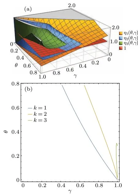
Fig.4.(a)The yellow,blue and green surfaces represent the values of η1(θ,γ),η2(θ,γ)and η3(θ,γ),respectively,as functions of parameters θ and γ.The red plane denotes z=1.Due to the limit of accuracy of the computer calculation,the images with k ≥4 cannot be plotted.(b)The blue,orange,and green curves represent η1(θ,γ)=1,η2(θ,γ)=1 and η3(θ,γ)=1,respectively.

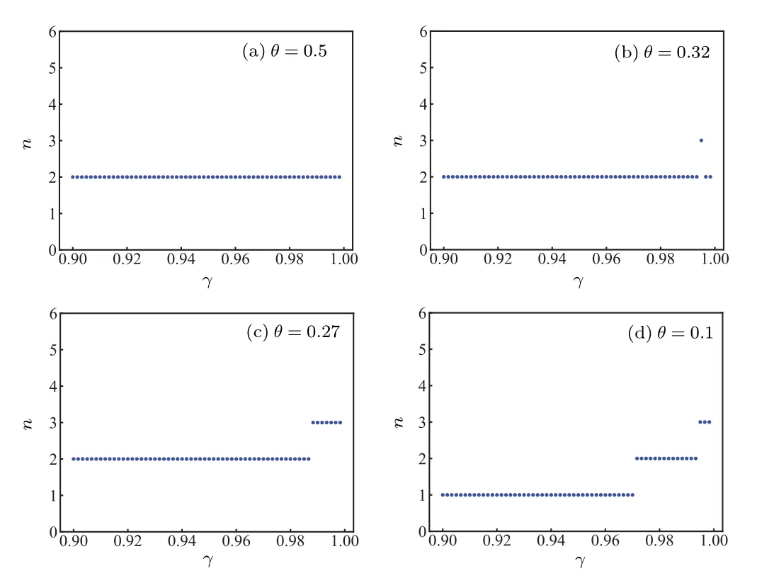
Fig.5.The value of the vertical axis n= is the maximal number of Bobs who can share nonlocality with Alice.

Case 2.0＜β1+β2＜2 andα=δ=γk=μk=1 for allk=1,2,...,n.In this case,we have

and obtain the corresponding sequenceas

where 0＜ηk?1(θ,β1+β2,ε)＜1 withη1(θ,β1+β2,ε)=forε ＞0,θ ∈(0,π/4] andβ1+β2∈[0,2].Letx=β1+β2.Ifηk(θ,x,ε)＜1,k= 1,2,...,n,andηn+1(θ,x,ε)≥1, then there are at mostnBobs sharing the nonlocality with Alice.We also plot the function values ofηk(θ,x) again whenε=10?5in Fig.6(a), and show the ranges of 0＜ηk(θ,x)＜1 in Fig.6(b), i.e., (θ,x) lies in the right-hand sides of each curves fork=1,2,3.

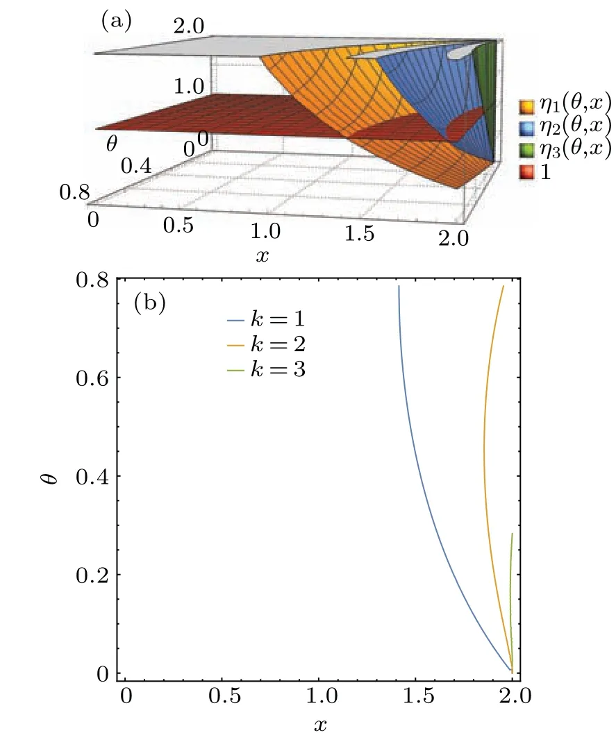
Fig.6.(a)The yellow, blue and green surfaces represent the values of η1(θ,x),η2(θ,x)and η3(θ,x),respectively,as functions of parameters θ and x.The red plane denotes z=1.Due to the limit of accuracy of the computer calculation,the images with k ≥4 cannot be plotted.(b)The blue, orange, and green curves represent the functions η1(θ,x) = 1,η2(θ,x)=1 and η3(θ,x)=1,respectively.

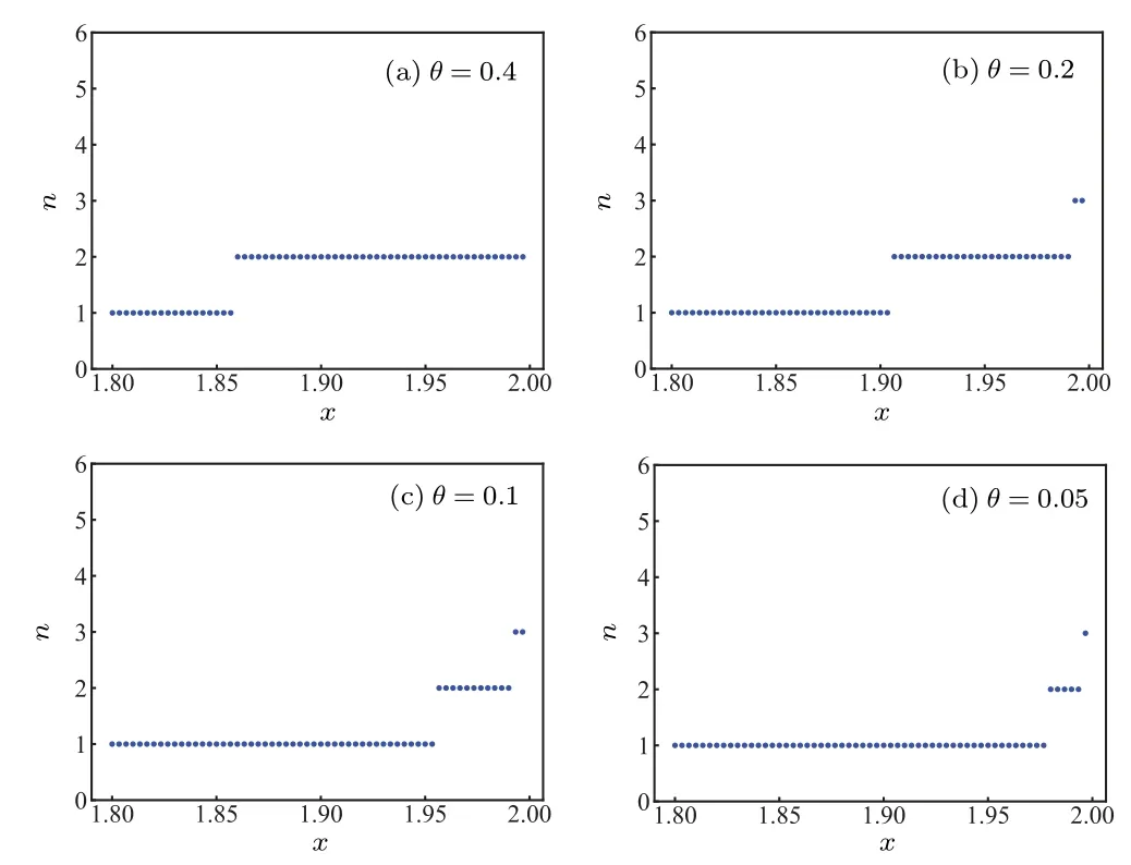
Fig.7.The value of the vertical axis n= is the maximal number of Bobs who can share nonlocality with Alice dependent on the noisy parameter x=β1+β2.When θ is fixed,n increases if x moves to 1.

Similarly, from Fig.6(b), the value ofcan be straightforward investigated when (θ,x) lies in the given region[0.4,π/4]×(0,1.8].For instance,=1 when(θ,x)=(0.4,1.5).In the region (0,0.4)×(1.8,2), we describe the change pattern ofdepending on the noise parameterx ∈(1.8,2) whenθis fixed as 0.4, 0.2, 0.1 and 0.05 respectively(see Fig.7).We see that whenθis given,increases ifxmoves from 1.8 to 2.On the other hand,in the four plots of Fig.7,the best persistency occurs whenθ=0.2.

4.The high-dimensional systems

In this section, we consider the persistency on sharing nonlocality noisily in the case of arbitrary finite-dimensional systems.The initial state with white noises is

with the noisy parameterν ∈[0,1].

We also affix white noises on measurements Eqs.(9)–(16).Then,when bothsandtare even,the noisy measurement strategies are defined as

forθ ∈(0,π/4]andk=1,2,...,n.When bothsandtare odd,a set of noisy POVMs are chosen to be

forθ ∈(0,π/4]andk=1,2,...,n.

Theorem 4 For the noisy initial state ?ρAB(1)in Eq.(42),assume that the Alice and Bobs perform noisy measurements Eqs.(43), (44)or(47), (48)and Eqs.(45), (46)or(49), (50),respectively.Ifβ1≥β2, then the expected CHSH value ofρAB(k)satisfies the inequality

whereθ ∈(0,π/4],ν,βi,γk,ηkandμk ∈[0,1] fori=1,2,k=1,2,...,n,andcjis the Schmidt coeffciient of|ψ〉forj=1,2,...,.A proof of Theorem 4 will be given in Appendix D.

By Theorem 4, we get a sufficient condition of persistency of sharing nonlocality noisily in the case of the arbitraryfinite dimension.

Theorem 5 For the noisy initial state ?ρAB(1)in Eq.(42),assume the Alice and Bobs perform noisy measurements as in Eqs.(43), (44)or(47), (48)and Eqs.(45), (46)or(49), (50),respectively,andβ1≥β2.Then there existnBobs sharing the nonlocality of the noisy initial state ?ρAB(1)with Alice if there existsε ＞0 such that

where

with

for anyk=1,2,...,n,andciis the Schmidt coeffciient of|ψ〉,i=1,2,...,.

Furthermore, we get another sufficient condition for the persistency of sharing nonlocality when part of the noises disappears,which extends the sufficient persistency condition for the two-qubit case to the arbitrary finite-dimension case.

Theorem 6 For the noisy initial state ?ρAB(1)in Eq.(42),let the Alice and Bobs perform noisy measurements in Eqs.(43), (44)or(47), (48)and Eqs.(45), (46)or(49), (50),respectively.Ifγn(β1+β2)ν=2 for somen, then there exist at leastnindependent Bobs who can share the nonlocality of the noisy initial state ?ρAB(1)with the single Alice for arbitrary given noisy parametersγk,μj ∈(0,1],k=1,2,...,n ?1 andj=1,2,...,n.

5.Discussion and conclusion

The aim of the paper is to determine how many Bobs can share the nonlocality with Alice at most in a noisy environment.For a given measurement strategy, two kinds of noises are considered on the initial states and measurements respectively.We establish a CHSH type inequality and obtain two persistency conditions of sharing nonlocality noisily.We also analyze the influence of the noises to persistency, that is, the maximal number of Bobs who can share with Alice.It is significant to find other anti-noise measurement strategy, which can result in the better persistency.

Note also that we consider only two different noise factors.From experimental perspectives,it would be more interesting to analyze errors that occur during physical implementation,such as the exponential decrease in coherence of quantum states.Apart from loss in coherence,nonlocality sharing becomes challenging due to photon loss, noise in photon detection,and many other factors.

Appendix A:Proof of Theorem 1

When the noisy measurement strategy Eqs.(27)–(32)are performed, then the CHSH value of Alice and Bob(k)can be computed as follows:

By using the Lüders rule,we have

where the third equation comes from

fori=0,1.Then,using Eq.(A2),we have

Similar to Eq.(A4),we get

By recursion,we get

It follows from Eqs.(A8)–(A11)and(A1)that

Proof of Theorem 1 For the case ofT(ˉρAB(1)) =diag(?αδ,αδ,δ),from Eq.(A12)we have

Using Eqs.(A13)–(A16)in Eq.(A12),we get

Appendix B:Proof of Theorem 2

From＞2,k=1,2,...,n,it is equivalent to

Define a function

Obviously,f(θ,α,δ,β1,β2,μ1,...,μk,γ1,...,γk,η1,...,ηk?1)＞0,then the inequality(B1)can be written as

we have

this implies that there existsε ＞0 such thatηk= (1+ε)f(θ,α,δ,β1,β2,μ1,...,μk,γ1,...,γk,η1,...,ηk?1).

Denote byXkthe set{ε,α,δ,β1,β2,μi,γi}ki=1.Furthermore,we define a sequenceηk(θ,Xk)as follows:

Ifηi(θ,Xi)＜1 fori=1,2,...,k ?1,then

Thus,ηk(θ,Xk)＜1 when

Set

We can rewrite inequality (B4) as (1+ε)(2k ?cos(θ)ak)＜bksin(θ)and get

The solution of inequality(B7)satisfies

where

for anyk=1,2,...,n,i.e.,θk ∈(arctan[xk2(ε)],arctan[xk1(ε)]).Therefore,if

Appendix C:Proof of Theorem 3

From assumption,γn(β1+β2)δ=2,denote byYkthe set of given nonzero parameters{ε,α,μs,γt}k,k?1s=1,t=1,one has

We can define a new sequence(pi(θ))iof the following form:

Appendix D:Proof of Theorem 4

In the following, we give a brief proof, which is similar to the proof of Theorem 1.When bothsandtare even,we use Eqs.(43),(44)and Eqs.(45),(46)as noisy measurements,we get

where

For the casek=1,we have

It follows from the Lüders rule, Eqs.(A3)–(A5) in Ref.[33] and Eqs.(D2), (D3), (D7)–(D9) that Eq.(D1) is transformed into

Then, we consider the case that bothsandtare odd,which is the most complex case.In this case,we use Eqs.(47),(48) and Eqs.(49), (50) as the noisy measurements for Alice and Bob(k),respectively.By calculation,we get

where

for someθ ∈(0,π/4]andk=1,2,...,n.Similar to the proof of Theorem 1,we can get

Combining the form of noisy initial state ?ρAB(1)with Eqs.(D11)–(D22)andβ1≥β2,Eq.(D1)can be rewritten as

For the case of even(odd)tand odd(even)s,it is analogous to prove inequality(51).

Acknowledgements

This work is supported by the National Natural Science Foundation of China (Grant Nos.12271394 and 12071336)and the Key Research and Development Program of Shanxi Province(Grant No.202102010101004).