Quantum estimation of rotational speed in optomechanics

Hao Li(李浩) and Jiong Cheng(程泂)

Department of Physics,Ningbo University,Ningbo 315211,China

Keywords: optomechanical system,Fisher information

1.Introduction

Quantum measurement is an important technology in quantum information science.[1-4]The bound of the detection accuracy is essentially due to Heisenberg uncertainty relationship.[5,6]Quantum parameter estimation can be used to find this limit in the precision of quantum measurement.[1,7]For a given measurement, the maximal achievable precision of the estimation is determined by the so-called Fisher information.[8]Many effective methods have been proposed to optimize measurements based on Fisher information, e.g.,Fisher-information-based estimation of optomechanical coupling strengths,[9]projective photon-counting measurement of single photons,[10]quantum estimation methods for quantum illumination,[11]and so on.

In the field of quantum measurement, the ability to detect the properties of a mechanical object at the quantum precision limit has attracted significant attention because it can show the boundary of quantum-classical transition,[12,13]macroscopic quantum effect[14-16]and so on.As a potential platform for precise measurement,[17-19]an optomechanical system has natural advantages[20-28]because a quantized light field is very sensitive to mechanical motion.[18,29-31]With the help of optomechanical coupling,a quantum detector can detect gravitational waves,[17,32-34]tiny masses,[35,36]tiny displacements,[37,38]and weak fields with greater precision than the classical detectors.[30]Among them,the measurement of angular velocity has attracted considerable attention,and is used as the basis of a gyroscope.[39,40]Meanwhile,a mechanical object is naturally sensitive to centrifugal force when rotating at a certain angular velocity.Related detection schemes have also been proposed in optomechanical systems.[40]By means of semi-classical treatment,the angular velocity can be introduced by the coefficients of the system operator,or by an effective drive.[41]

The detection limit of the system has not yet been fully discussed in these studies.We note that the combination of the optomechanical system with QFI allows us to estimate the parameters of the system.In Ref.[9],the designed quadrature measurements allow very accurate estimation of optomechanical coupling strengths.This offers a possibility to estimate the angular velocity by using quantum metrology with the platform of optomechanical system.QFI can be used to quantify this estimation and give the limit.Therefore,in this study we use QFI to investigate the limit of optomechanical system in angular velocity detection.

This paper is organized as follows.In Section 2, we introduce the system and derive the dynamical evolution of the Hamiltonian.In Section 3, we discuss the relationship between covariance matrix and QFI under Gaussian measurement.The numerical results and the corresponding discussion are given in Section 4.Finally, a summary is given in Section 5.

2.Model

We consider a cavity optomechanical system that consists of a Fabry-P′erot cavity with frequencyωcand a mechanical resonator with frequencyωm.The cavity is driven by a coherent laser with driving strengthεand center frequencyω0.The system is fixed on a rotating table with angular velocityΩ(see Fig.1).The Hamiltonian of the system reads[42,43]

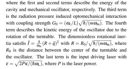
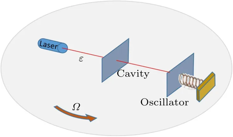
Fig.1.Schematic diagram of optomechanical gyroscope.A cavity optomechanical system is placed on a rotating platform with its input end located at the center of the platform.The platform is rotating with angular velocity Ω.

In the frame rotating at the laser frequencyω0, we can obtain the following quantum Langevin equations:[44-46]

The system is stable and reaches its steady state when all of the eigenvalues ofAhave a negative real part.The stability conditions can then be derived by applying the Routh-Hurwitz criterion.From now on, we assume that the stability conditions are satisfied.If the mechanical quality factor is large enoughQ=ωm/γm?1,then ?ξ(t)is delta-correlated[45]

whereDis the noise matrix

The parameter to be measured,i.e.,Ω,is encoded in the drift matrixA, which determines the steady-state covariance matrix.Therefore, by detecting the output field, one can obtain information about the covariance matrix, which may help us to estimate the value of the angular velocityΩ.

Now we take the covariance matrix of our model in this result.The solution of Eq.(8)can be expressed in the following matrix form:

Hereσm(σL)corresponds to the covariance matrix of the mechanical (optical) subsystem, whileσcbrings about the optomechanical correlations.In this system, the output optical signals can easily be measured through optical homodyne detection, and therefore we can use the input-output relationshipto obtain the optical output matrixσL,out.

3.QFI of optomechanics with Gaussian measurements

In quantum metrology,the Cram′er-Rao bound[48]is one of the most important results in parameter-estimation theory.For an unbiased estimator, the Cram′er-Rao bound of the parameterθto be estimated reads

wherenis the number of measurements.For continuous variables,F(θ)reads

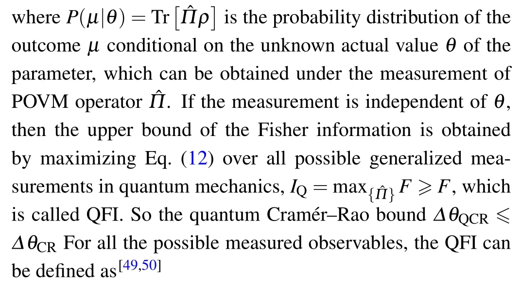
whereLis the symmetric logarithmic derivative(SLD)operator,which satisfy

According to the Gaussian measurements method of QFI,[51]we can derive the following single-mode Gaussian QFI ofΩ(the detailed derivations are given in Appendix A):

Thus, the parameter measurement precision can be evaluated through Eq.(15) when the covariance matrixσL,outis determined.We know that the covariance matrix is a positive semidefinite matrix and its determinant is the product of the eigenvalues of the matrix.Note that the mean values of the linearized fluctuation Eq.(3) is zero.Meanwhile, the system decoherence dynamics are certainly affected by the optomechanical coupling.Thus, according to the Heisenberg uncertainty relation,detσL,out≥1/4.The denominator of Eq.(15)will remain greater than zero.From the above analysis and Eq.(15), it can be found that if the input state is a squeezing state,then QFI can be further improved.The information of the mechanical oscillator is transmitted to the photon via the optomechanical coupling.WhenΩincreases,the number of photons in the cavity increases correspondingly,and consequentlyδ?Xandδ?Yalso increases.The partial derivative of the covariance matrix with respect toΩ, namely,?ΩσL,out, then increases.This is the reason why the measurement accuracy ofΩcan be improved.Since?ΩσL,outshould be greater than zero,this guarantees the non-negativity of QFI in Eq.(15).

4.Rotational speed estimation in optomechanical system

In this section, we numerically study the impact of system parameters on QFI.By solving the Lyapunov equation,the output optical covariance matrix is obtained,and then QFI can be determined through Eq.(15).Figure 2 shows the density plot of QFI varies with the laser powerPand cavity detuningΔ.To clearly show the distribution characteristics of QFI, we only show the regime thatIQ＞0.1 (i.e., the iridescence line between green and white areas).The green area represents the stability regime of the system, while the white area represents the unstable regime.By changing the optical dissipation rateκ,the stability regime has changed markedly,and we note that the large values of QFI always appear at the boundary of the stability regime.Near the unstable regime,the nonlinear effect of the system plays a leading role, which greatly affects the value of QFI.Meanwhile, in the unstable regime, the assumption of steady-state covariance matrix is not valid and the covariance matrix changes abruptly at the boundary.This results in the formation of extreme values of QFI at the boundary.We can also see that the QFI has a lot of local optimum points at the boundary.This indicates a way to improve measurement accuracy,i.e.,driving the system close to the unstable regime and finding the global optimum value for QFI.Comparing Figs.2(a) and 2(b), we find that we can improve the QFI of the angular velocity measurement by increasing theQfactor of the cavity.In Fig.2(c),we present the partially enlarged drawing of Fig.2(a), which clearly shows the behavior of QFI near the boundary.This also provides us with a reliable range of parameters for achieving large values of QFI.We plot Fig.2(d)by fixing the cavity detuning along the boundary.The small peak in(d)indicates the local optimal value of QFI.For our numerical analysis,we take experimentally feasible parameters,[52]which arem=6 ng,L=25 mm,ωm/2π=2.75×105Hz,γm=10-5ωm,ωc=4.8×102THz.In addition, we assume that the angular velocity to be measured isΩ=35 Hz,and the distance between the center of the turntable and the oscillator isR0=5L.

Fig.2.(a)-(c) Density plot of QFI as a function of laser power P and cavity detuning Δ.(d) QFI as a function of laser power P when Δ is fixed along the boundary.We set m=6 ng, R0 =5L, L=25 mm,ωm/2π =2.75×105 Hz,γm=10-5ωm,ωc=4.8×102 THz, ˉnth=100,and the rotational speed Ω = 35 Hz.In panels (a) and (b) we keep κ/ωm = 0.05, and 0.5 respectively.The partial enlarged drawing of panel(a)is plotted in panel(c)for Δ ～0.6.

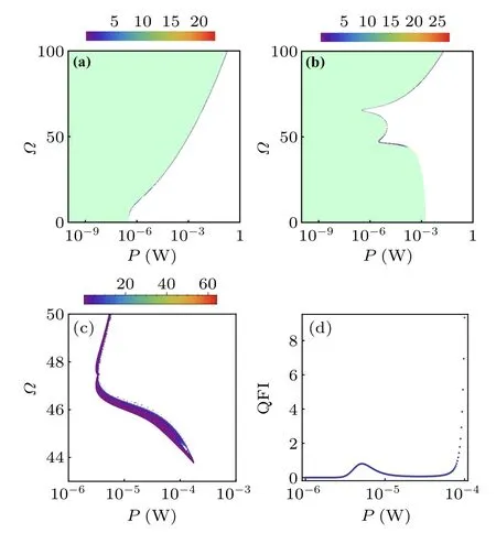
Fig.3.(a)-(c)Density plot of QFI as a function of the laser power P and angular velocity Ω.(d) QFI as a function of laser power P when Ω is fixed along the boundary.The parameters are the same as in Fig.2.In panel(a)we keep Δ =-1 and in panel(b)Δ =1.The partially enlarged drawing of panel(b)is plotted in panel(c)for Ω ～46 Hz.

In the following,we investigate the sensitivity of the angular velocity.We use blue and red detuned lasers to pump the cavity, and the results are shown in Fig.3.In Fig.3(a),the laser is blue detuned, and we can see that the steadystate region increases asΩgets larger.In this situation, forΩ ＜50 Hz,the required maximum laser power isP ≈1 mW.In the high rotational speed case, the blue detuned laser is no longer valid and one should modulate the laser to the red detuned regime, which is shown in Fig.3(b).In (b),the high rotational speed can be measured on the mW scale,while forΩ ＜50 Hz the accuracy of the measurement decreased significantly, i.e., QFI＜0.1.The results of Fig.3 can be understood very clearly because the effective detuning.For the parameters under consideration,G0R ?1.Then, increasing the angular velocity will effectively decrease the effective detuning, which means that the appropriate regime for our detection scheme is to keepˉΔ ≈-1.We also present the partially enlarged drawing of Fig.3(b)in Fig.3(c),which gives us a clear parameter regime for achieving large QFI.The local optimal behavior of QFI is also observed in Fig.3(d),where the angular velocity is fixed along the boundary.

5.Conclusion

In conclusion, we have studied the QFI of the rotational speed in an optomechanical system.We derived the explicitly single-mode Gaussian QFI for arbitrary angular velocity.Using this result,we find the way to maximum the value of QFI,i.e., driving the system close to the unstable boundary.Our results show that the optomechanical system can be used as a gyroscope,detecting the rotational speed with high precision.

Appendix A:QFI for Gaussian state

In this appendix, by using the approach proposed in Ref.[51],we will give a detailed derivation of our main result,i.e., Eq.(15).For n-mode Gaussian states, the symmetrically ordered character function is

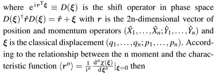
By using the exponential expansion and taking the first two moments,we get

Meanwhile,one can easily find that

To calculate the traces above, we use the following partially symmetrically ordered characteristic function:

where

Substituting Eq.(A10)into Eqs.(A8)and(A9),then

we have the following matrix forms:

This is an implicit matrix equation.One solution is to use canonical transform to take it into the diagonal representation.Here we define a matrixSsatisfyingSJST=J,then

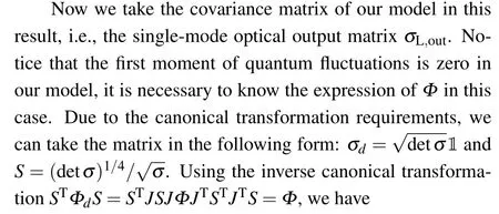
whereD=diag(d1,d2,...,dn)≥1 is a diagonal matrix.Since the covariance matrixΓis canonical matrix

then

where the defined symbolΦd=JSJΦJTSTJT, Notice thatΓdandJare commuted with each other

which can be solved explicitly

An inverse symplectic transformation can transform it back toΦ.By putting Eq.(A10)into the definition of QFI,we have

note thatJ?θσJT?θσ=det?θσ1,therefore

For the first term in the trace, notice that we only sum over diagonal elements andσdis diagonal,and then we have

The last step in the above equation uses the rotation property of trace,and finally we get

Acknowledgments

Project supported by the National Natural Science Foundation of China (Grant Nos.11704205 and 12074206), the National Natural Science Foundation of Zhejiang Province(Grant No.LY22A040005), and K.C.Wong Magna Fund in Ningbo University.