Turing pattern selection for a plant–wrack model with cross-diffusion

Ying Sun(孫穎), Jinliang Wang(王進良),?, You Li(李由), Nan Jiang(江南), and Juandi Xia(夏娟迪)

1LMIB and School of Mathematics and Science,Beihang University,Beijing 100191,China

2College of Science,Beijing Forestry University,Beijing 100083,China

Keywords: plant–wrack model,cross-diffusion,Turing instability,pattern selection,amplitude equation

1.Introduction

As one of the important branches of nonlinear science,pattern dynamics aims to explore the basic dynamic laws that exist among various ecological systems.[1,2]Patterns are nonuniform macroscopic structures with a certain regularity in space or time and are ubiquitous in nature.[3]Therefore,understanding the causes and mechanism of pattern production is of great importance for uncovering the mystery of natural formation.[4–7]

Plant and wrack are of great significance for protecting the ecology of freshwater wetland.For example, the spatial distribution of plant and wrack can provide a habitat for small animals.[8]In this ecosystem,we observe that little haystacks grow on top of the old ones; these may be induced by diffusion and the interaction of promotion and inhibition of plant and wrack.Therefore, Koppel proposed a reaction–diffusion model

to study and explain the regular spatial patterns.[9]

The biological meanings of the variables and parameters of system(1)are as follows:P(t,x,y)andW(t,x,y)are plant biomass and wrack biomass at timetand spatial position(x,y),respectively;iPWdescribes the inhibition effect of wrack on plant growth;k3stands for the level of plant biomass at which inhibition is reduced by half;iis a constant that converts wrack biomass into specific plant growth inhibition;the positive numberbindicates the decay rate of wrack;srepresents the plant decay rate;dPanddWare the positive self-diffusion coefficients of plant and wrack, respectively.Ωis a bounded domain in R2with the smooth boundary?Ωand ?2represents the Laplacian operator in two-dimensional space.nis the outward unit normal vector on?Ωand 1/?ndenotes the operator of the directional derivative along the directionn.

Many researchers have investigated system (1).Yu derived the mathematical expressions of Hopf bifurcation and the Turing bifurcation boundary and located the Turing bifurcation domain in parameter space; it was found that the typical plant dynamics involves the formation of isolated groups,namely spots, labyrinths and a mixture of stripes and spots,which explained the appearance of the Turing pattern.[10]Liuet al.also gave the Turing region in parameter space,and discovered the self-organization behavior between plant and wrack,which induced the formation of a spot pattern.[11]Wanget al.carried out theoretical analysis and numerical simulation on model(1)and found that the layer structure of the pattern was induced by the simultaneous instability of the periodic solution with a large amplitude and equilibrium point.[12]Houet al.studied pattern formation mechanisms arising from the interactions between plant and wrack, and gave the conditions for the existence of the patterns.[13]Liet al.investigated the spatiotemporal patterns of a freshwater tussock sedge model(1)with discrete time and space variables.They obtained that stable homogeneous solutions can experience Turing instability under certain conditions.[14]For more works about model(1),one can refer to Ref.[15]and the references therein.

Most of the work on biological models has focused on self-diffusion; however, cross-diffusion also plays an important role in many biomasses and is more practical.Kerner mentioned the practical implications of cross-diffusion, and subsequently cross-diffusion in biological models attracted the attention of many scholars.[16]So far,cross-diffusion has been applied to population dynamics,competitive population models and prey–predator models,etc.[17–26]Iida and Banerjee and their colleagues considered the effect of movement of individual prey on predator populations, and introduced a crossdiffusion term of the ?2(uv) type into their model.[27,28]For more about the effects of cross-diffusion, one can refer to Refs.[29–37].In the biological sense, there exists crossdiffusion between plant and wrack,as the two can promote or inhibit each other.Moreover, few results have been reported regarding cross-diffusion and pattern selection in the plant–wrack model,so we introduce a cross-diffusion term ?2Pinto the second equation of model(1), and the cross-diffusion coefficient is denoted byd:

In this paper,our main aim is to study the pattern selection of system (3) through multiple-scale analysis theory, which can give not only the general form of the amplitude equation near the bifurcation point but also determine the corresponding relationship between coefficient and control parameter of the system.Thus, we can know which control parameters of the system are effective.Then we can estimate the effective region of the amplitude equation and study the specific process of the pattern formation in a system with change in the control parameters.

The paper is organized as follows.In Section 2, we investigate the system and conclude that cross-diffusion leads to Turing instability.In Section 3, we obtain the amplitude equation of the Turing pattern at the Turing bifurcation point and obtain the theorem of pattern selection.In Section 4, we verify the correctness of our theoretical analysis through numerical simulations.Finally, in Section 5, a brief conclusion is presented.

2.Turing instability of the system

In this section, we focus on the Turing instability of the system (3).Before starting our research, we first require that the positive equilibrium of the ordinary differential equation(ODE)system is stable.

We consider the ODE system associated with system(3),namely, the non-spatial system in the absence of diffusion terms

In the following, we perform stability analysis for system(4)and obtain the stability theorem.

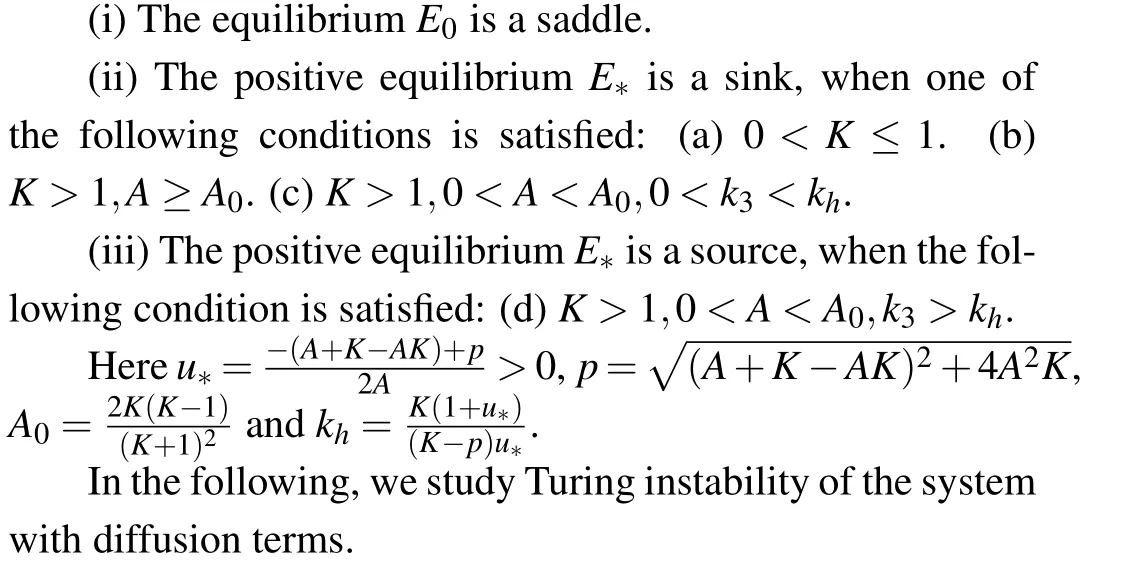
Theorem 1[Wanget al., 2019] There are two nonnegative equilibriaE0=(0,0)andE*=(u*,u*)in system(4).

2.1.Turing instability for a system with self-diffusion

In this part,we will discuss the Turing instability for the system(3)with self-diffusion(i.e.,d=0),that is

Linearizing system(5)at the positive equilibriumE*,we have

where

Obviously, the trace and the determinant have the following forms:

Next,we consider the solution of the system(6)with the following form:

wherek=(kx,ky),k·k=k2,r=(x,y)represents the spatial vector in two-dimensional space,kxandkyare the wave numbers of the solution,λrepresents the growth of disturbance in timetand i represents the imaginary unit, that is, i2=-1.Now,substituting Eq.(8)into Eq.(6),we have

where

In the following,we give stability results for the system(5).

Theorem 2

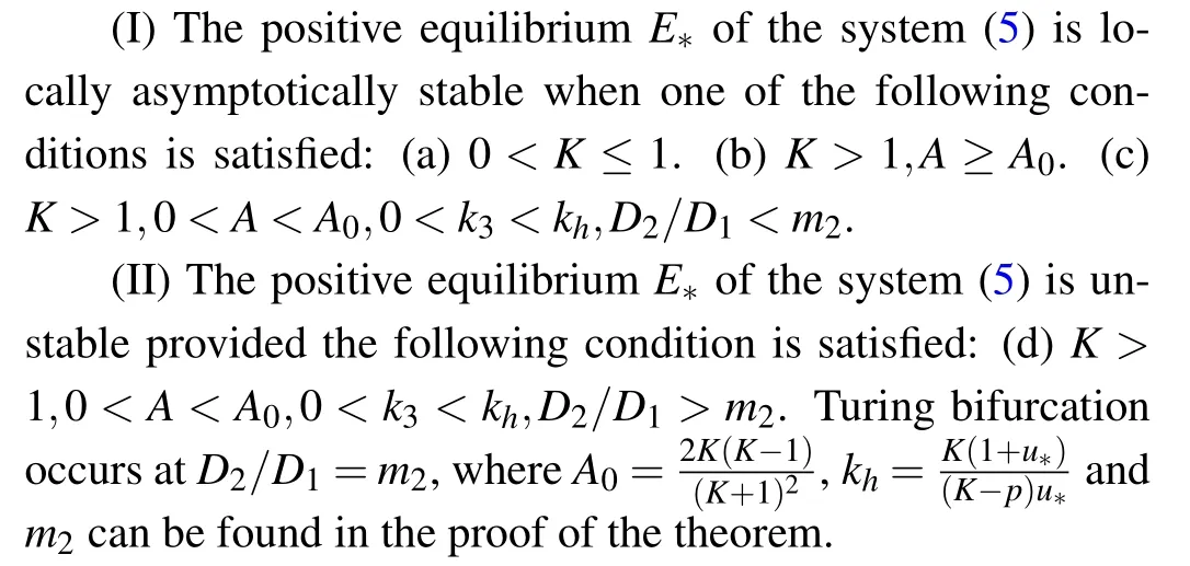
ProofSuppose condition(ii)of Theorem 1 holds.When condition (ii-a) or (ii-b) is satisfied, thena11≤0.So Det[J(k)]＞Det(JE*)＞0 and the equilibriumE*is still stable.When condition (ii-c) of Theorem 1 is satisfied, then 0＜a11＜1.We want to determine the sign of Det[J(k)],which can be viewed as a quadratic trinomial ofk2.The discriminant

wherea11,a12,a21,a22are given by Eq.(7).Clearly-a11a22+ 2a12a21＜0, and (a11a22- 2Det(JE*))2-(a11a22)2＞0.Thus,Δcan be viewed as a quadratic trinomial ofD2/D1,and it has two positive roots

wherem0=-a22/a11＞0.

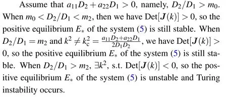
Assume thata11D2+a22D1≤0, namely,D2/D1≤m0.Then we have Det[J(k)]＞Det(JE*)＞0, so the equilibriumE*is still stable.

2.2.Turing instability for systems with self-diffusion and cross-diffusion

In this section, when a system with a self-diffusion term is stable, we study the Turing instability induced by crossdiffusion in the system(3).Linearizing system(3)at the positive equilibriumE*,we have

Considering the form of the solution

Next, substituting Eq.(11) into Eq.(10), we obtain the dispersion relation

where

Based on the condition of self-diffusion stability,together with the analysis of its stability when cross-diffusion is added,we can obtain the following results:

Theorem 3Suppose condition (I) of Theorem 2 holds.Then we have

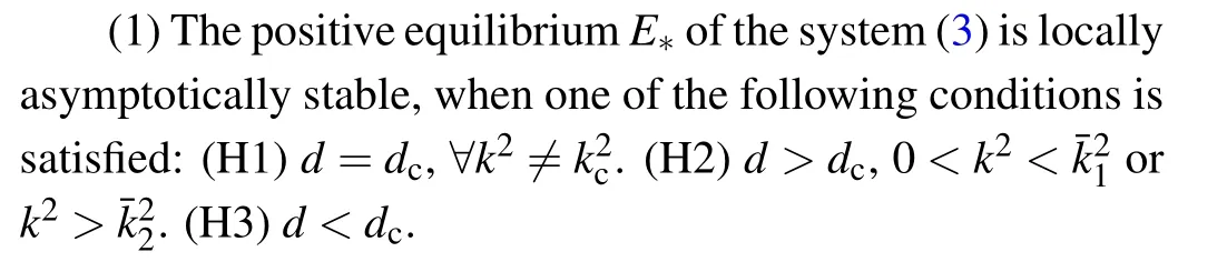
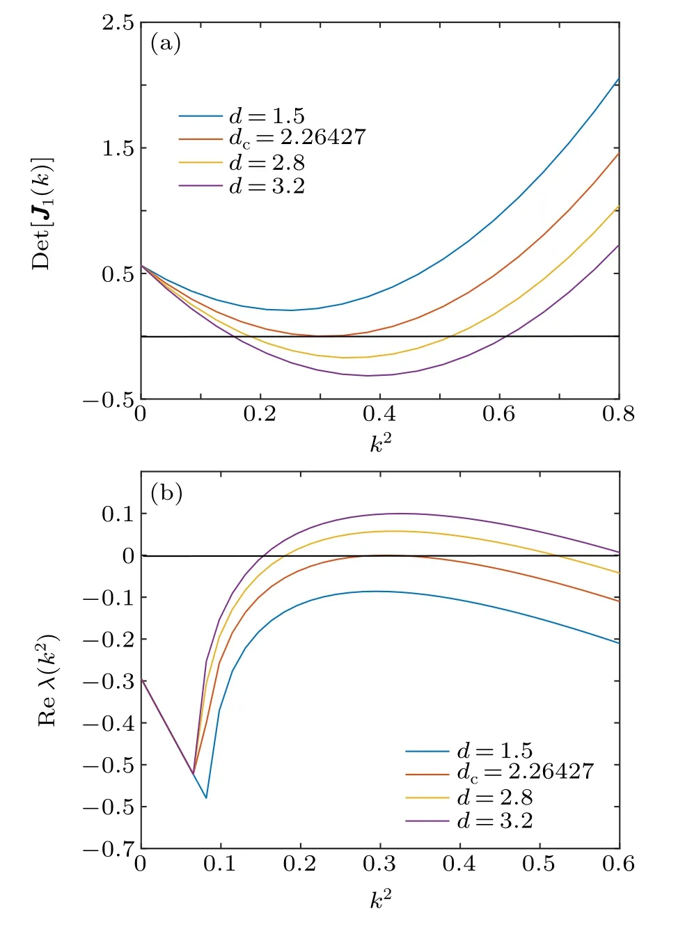
Fig.1.(a)Function images of Det[J1(k)]with k2 under different crossdiffusion coefficients d.(b)The real part of the largest value as a function of k2,where dc=2.26427(orange),d=1.5(blue),d=2.8(yellow)and d =3.2 (purple).The other parameter values are selected as k3 =1.5,A=0.8,K=10,D1=1 and D2=6.

and setq=-γd+δ,whereγ=-a12,δ=-a11D2-a22D1.Then substituting it into the second equality of Eq.(13):

Clearly,equation(14)has a negative root,denoted byq*,then we define

Whend=dc,namelyq=q*,we obtain Det[J1(kc)]=0,then Det[J1(k)]＞0,?k2/=k2c,and the positive equilibriumE*of the system(3)is still stable.

Whend ＞dc,namelyq ＜q*＜0,we get Det[J1(kc)]＜0,then it has two positive roots

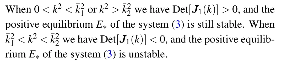
Whend ＜dc,namelyq*＜q ＜0,we have Det[J1(k)]＞0,and the positive equilibriumE*of the system(3)is still stable.

In the next section,we discuss the amplitude equations of Turing patterns atd=dc.

3.The amplitude equations of the Turing pattern

In this section,we think about the amplitude equations of Turing pattern atd=dc.Considering system(3)that includes self-diffusion and cross-diffusion terms,we use three steps to get the amplitude equations.

Step 1 We consider the perturbation solution(u-u*,vu*)Tof system(3),and we have

where

LetU=(u,v)T,and system(15)can be transformed into the following system:

where

Let

Step 2 We expand the solution of system(3)with a small parameterεas follows:

where

Next,we separate the time scale for system(16):

then

We substitute Eqs.(17)–(21)into Eq.(16), and the following equations can be obtained:

The order ofε:

The order ofε2:

The order ofε3:

We can see thatLcis the linear operator close to the onsetd=dcfor the order ofεas in Eq.(22).The form of the solution is as follows:

The zero eigenvector ofL*cis

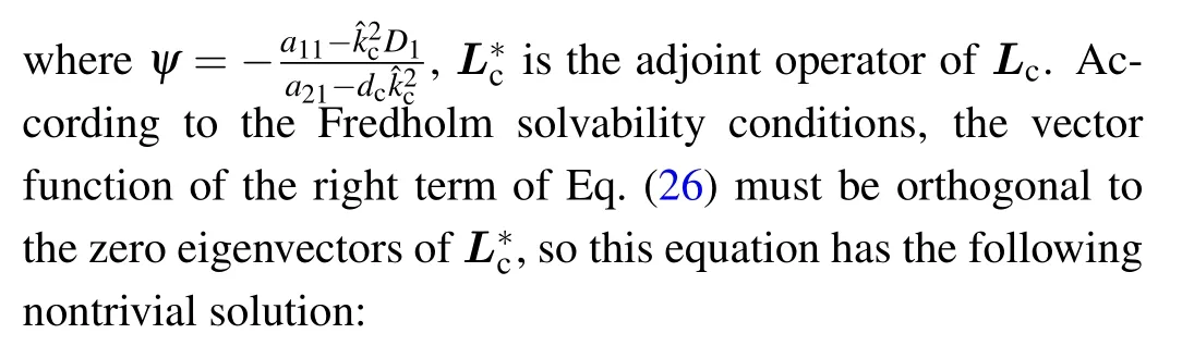
Substituting Eq.(25)into Eq.(26),we get

where

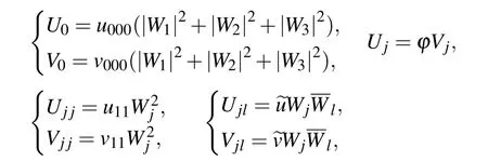
For the order ofε3:

The coefficient of the term eik1·rin Eq.(31)is

where

We can write one of the equations as follows,then it is easy to get the other equations by transforming the subscripts:

Step 3 Supposing

according to Eq.(21)we have the amplitude equation ofAj:

From the above conclusions, we get the amplitude equations as follows:

where

Next,we analyze the stability of the amplitude Eq.(34).Each amplitude in the above equations can be expressed as follows:

whereρj=|Aj|represents mode andθjrepresents the corresponding phase angle.Substituting Eq.(35)into Eq.(34)and separating the real and imaginary parts for comparison, one can obtain

whereθ=θ1+θ2+θ3;clearlyμ ＞0.To guarantee the existence of the steady-state solution of Eq.(36), the coefficients ofg1andg2must be positive.Moreover,g2＞g1＞0.

Theorem 4

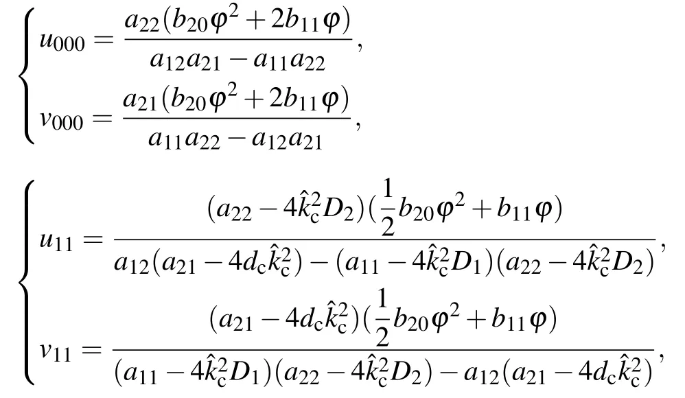
(1)The homogeneous steady state:

which is stable whenμ ＜0 and unstable whenμ ＞0.

(2)Stripe patternS:

(3)Hexagonal patternH0orHπwithθ=0 orθ=π:

is always unstable wheng2＞g1andμ ＞μ2.

To sum up, when we change the value of the crossdiffusion coefficientdand fix the other parameters in the system(3),we can calculate the value ofh,μ,μ1,μ2andμ3,and we haveμ1＜0＜μ2＜μ3.

Theorem 5

(1) Ifh ＞0, then the hexagonal pattern is shown asH0(θ=0), whileHπis always unstable; ifh ＜0, then the hexagonal pattern is shown asHπ(θ=π),whileH0is always unstable.

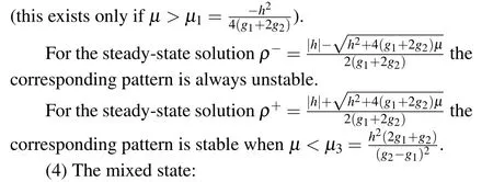
(2)Whenμ ∈(μ1,0),the homogeneous steady state and the hexagonal pattern are stable;whenμ∈(0,μ2),the hexagonal pattern is stable,but the homogeneous steady state and the stripe pattern are unstable; whenμ ∈(μ2,μ3), the stripe pattern and the hexagonal pattern are stable,but the homogeneous steady state is unstable;whenμ∈(μ3,∞),the stripe pattern is stable, but the homogeneous steady state and the hexagonal pattern are unstable.

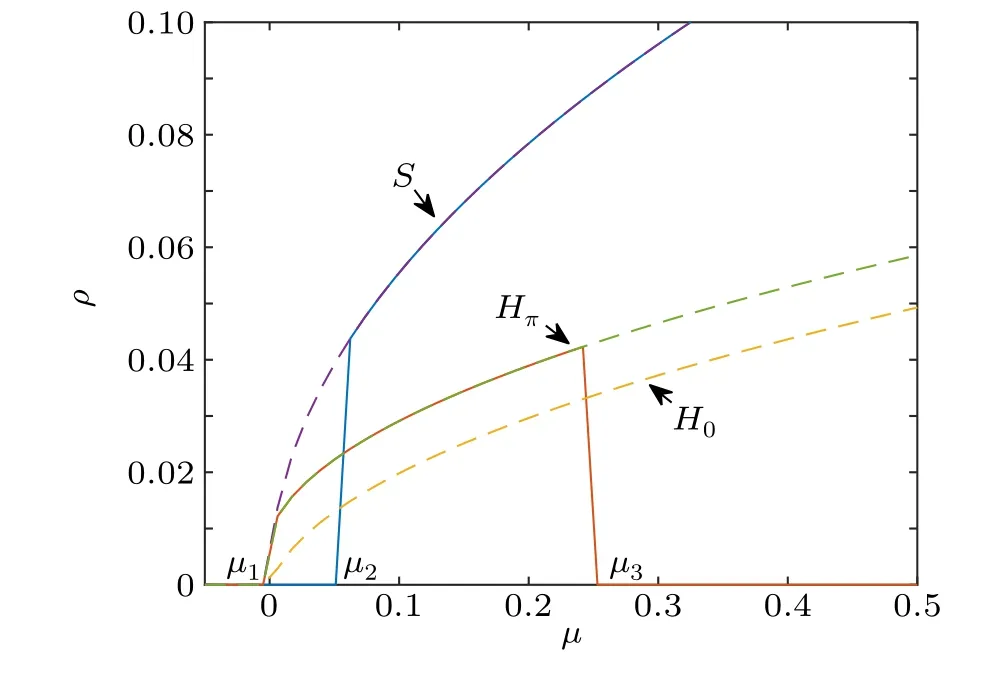
Fig.2.The bifurcation diagram of the amplitude Eq.(34).Here S represents the stripe pattern; H0 represents the hexagonal pattern with θ =0;Hπ represents the hexagonal pattern with θ =π.The solid line is the stable state;the dotted line is the unstable state.

4.Numerical simulation

In this section, we use MATLAB to simulate system (3)in two dimensions.To analyze the dynamic behavior of the system, we study it on discrete grids of 100×100 with Neumann boundary conditions, and take the space step as 1 and the time step as 0.01.As is well known,the system dynamics are determined by the initial conditions.The species distribution will always be uniform if the initial spatial distribution of plant and wrack is uniform;however,we are interested in random perturbations of the initial conditions around a uniform distribution of the unique positive equilibriumE*=(u*,u*).In the numerical simulation,we observe different types of patterns, and the distributions of plant and wrack are always the same types of patterns.Therefore, we only show the pattern formation for plant biomassu(t,x,y)in our numerical simulations.

In the following, we show the different types of patterns due to the variation of the cross-diffusion coefficientd.Among the parameter values of system (3), we selected the three sets of parameter values shown in Table 1.Then we obtained the unique positive equilibriumE*=(1.8642,1.8642)of system (3) and the critical value of the Turing bifurcation asdc=2.26427.We geth=-1.6092,g1=32.4881,g2=70.3498,μ1=-0.0037,μ2=0.0587 andμ3=0.2445.From the previous analysis, we know that the values in Table 1 satisfy condition(2)of Theorem 3,namely,the only positive equilibriumE*is unstable and Turing instability occurs atd ＞dc.

First,we taked=2.3238,satisfying this parameter condition.Condition(2)of Theorem 3 holds and Turing instability occurs.Further,we can calculate that at this pointμ=0.0263 belongs to (0,μ2), and according to the conclusion of Theorem 5, system (3) will form a hexagonal pattern and be stable.From the simulations,we can see that a hexagonal pattern gradually forms as timetincreases(see Fig.3).

Fig.3.(a)t =0, (b)t =1000, (c)t =4000, (d)t =6000, (e)t =9000,(f)t=12000.The system parameters are listed in Table 1.

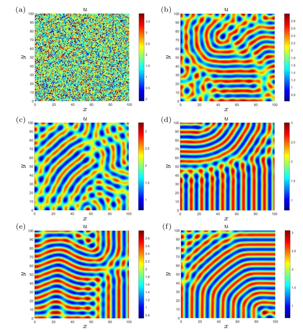
Fig.4.(a)t=0,(b)t=500,(c)t=1000,(d)t=3000,(e)t=8000,(f)t=10000.The system parameters are listed in Table 1.

Next, we taked=2.4728, which satisfies condition (2)of Theorem 3, at which point Turing instability occurs.It is calculated thatμ=0.0921 belongs to (μ2,μ3), and according to the conclusion of Theorem 5,the hexagonal pattern and stripe pattern are stable.In the numerical simulations,as timetgrows,We can observe a mixture state of hexagonal and stripe patterns,as shown in Fig.4.

Finally, we taked=2.8503, and satisfying this parameter condition,condition(2)of Theorem 3 holds,which tells us that Turing instability will occur andμ=0.2588 belongs to(μ3,∞).We get a stable stripe pattern according to the conclusion of Theorem 5.By numerical simulation,we find that the stripe pattern gradually forms as timetincreases(see Fig.5).

In summary, the numerical simulation verifies our theoretical results.

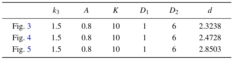
Table 1.Parameter values in Figs.3–5.

Fig.5.(a)t=0,(b)t=500,(c)t=1000,(d)t=3000,(e)t=8000,(f)t=12000.The system parameters are listed in Table 1.

5.Conclusion

In this paper we study the Turing instability and pattern formation mechanism of a plant–wrack model with both self-diffusion and cross-diffusion terms, and conduct theoretical analysis and numerical simulation of this model.It is found that the formation of spatial patterns induced by cross-diffusion has an important influence on pattern selection.The theoretical and numerical simulation results show that the plant–wrack system (3) with cross-diffusion exhibits a very rich dynamic behavior.As the cross-diffusion coefficientdchanges, the system will have different types of pattern structure: when the cross-diffusion coefficientdbelongs to (dc,dc+dcμ2), the distribution of plant presents hexagonal patterns(see Fig.3).Whendbelongs to(dc+dcμ2,dc+dcμ3), mixtures of hexagonal and stripe patterns appear (see Fig.4).When the cross-diffusion coefficientdbelongs to(dc+dcμ3,∞),we obtain stripe patterns(see Fig.5).

Acknowledgments

Project supported by the National Natural Science Foundation of China (Grant Nos.10971009, 11771033, and 12201046),Fundamental Research Funds for the Central Universities (Grant No.BLX201925), and China Postdoctoral Science Foundation(Grant No.2020M670175).