Soliton propagation for a coupled Schr¨odinger equation describing Rossby waves

Li-Yang Xu(徐麗陽), Xiao-Jun Yin(尹曉軍), Na Cao(曹娜) and Shu-Ting Bai(白淑婷)

College of Science,Inner Mongolia Agriculture University,Hohhot 010018,China

Keywords: Hirota bilinear method,Schr¨odinger equation,soliton solution,Rossby waves

1.Introduction

In the last few years,Rossby waves have been the subject of our study.[1–3]The result based on the single-layer quasi geostrophic vortex equation[4]is an approximate result.For the actual ocean and atmosphere,because of the inhomogeneity of fluid density and the multi-physicality of mixed fluid,the two-layer fluid pattern is real existence.In addition, the two-layer fluid can better fit the actual atmosphere and ocean,because they play an important role in the ocean atmospheric fluctuation, especially in the deep-sea internal wave theory.The two-layer fluid model attracts much attention from scholars.For example,Yanget al.derived a set of time-space fractional coupled generalized Zakharov–Kuznetsov equations to explore the Rossby waves’property in two-layer fluids and obtained group solutions for them,[5]derived(2+1)-dimensional coupled Boussinesq equations describing Rossby waves in a two-layer cylindrical fluid and gave their exact solutions,[6]then derived coupled Kadomtsev–Petviashvili equations and gave their soliton solutions.[7]We notice that a Boussinesq equation of Rossby waves can be written as

wherexis the coordinate in latitudinal direction,zrepresents the coordinate in vertical direction;tdonates the time;uandwrepresent the velocities inxandzdirections,respectively;T′is the temperature perturbation.The perturbation pressure,density, zonal mean background temperature, gravitational constant,dry adiabatic lapse rate,and moist lapse rate are all donated byp′,ρ0,T0,g,γd,andγ,respectively.[8]

A coupled nonlinear Schr¨odinger(CNLS)equation[9]can be derived from the Boussinesq equation and can also be obtained from the literature,[10]that is,

the coefficientsα1andα2are dispersion coefficients,σ1andΓ2are Landau constants,Γ1andσ2are interaction coefficients.[9]Equation (2) can be obtained through optical waves[11]or large-scale Rossby waves.[9]

Research of the CNLS equation in aspects of physics and mathematics is of continuous interest because of the science applying in many fields such as nonlinear optics,[12–15]optical communication,[16–19]Bose–Einstein condensates,[20,21]and plasma physics.[22,23]

The system (2) has received great attention by many researchers.For example, the symmetries and symmetry reductions have been obtained, and some exact solutions have been given by using the classical Lie group approach,[8]while there is little analysis of the solutions for the equation.In Ref.[24], two CNLS equations which are also a special case of the system(2)were discussed about the integrability properties through Painlev′e analysis.At the same time, their accompanying B¨acklund transformation and the Hirota bilinear forms were build.In Ref.[25],Louet al.also investigated the system’s Painlev′e integrability.

Introducing a transformation

whereB=B(X,T).

Using the above transformation, letu(X,T)=A1(X,T),v(X,T)=B(X,T),the system(2)is transformed into

By using the inverse scattering transform approach,equation(4)is typically not integrable,with the exception of high symmetry instancesα1=α2=±1,σ1=Γ2=σ2=Γ1=±1,a periodic travelling wave solution in terms of the Weierstrass function has been obtained.[26]Then, Makhankov found that equation(4)is completely integrable and gave the corresponding Lax pair.[27,28]

Whenα1=α2= 1, equation (4) reads the Manakov model.[29]Whenσ1=Γ2=σ2=Γ1=1, equation (4) reads the focusing Manakov model.Whenσ1=Γ2=σ2=Γ1=?1,equation (4) is of the defocusing Manakov model.Whenσ1=Γ2=1,σ2=Γ1=?1 orσ1=Γ2=?1,σ2=Γ1=1,equation (4) is of the mixed Manakov model.[30,31]The focusing Manakov model has bright-bright solitons.[29]Brightdark and dark-dark soliton solutions are supported by the defocusing Manakov model.[32]However,in the mixed case,the Manakov model admits bright-bright soliton,bright-dark soliton, and dark-dark soliton solutions.[17,18,30]Feng considered a generalN-soliton solution to a vector Schr¨odinger equation,following that, extended to the multi-component case, of allfocusing,all-defocusing and mixed types by the KP hierarchy reduction approach.[31]Researchers have used different methods to solve the equations in the literature.[17,18,30,31]However,as far as we are aware,they have not provide the three-solution solutions and do not work on the two-soliton and three-soliton solutions’ propagations.There are other methods for solving nonlinear equations,[33]but recently the Hirota bilinear method seems to be used more frequently.[34–42]Some scholars have recently focused on soliton solutions,[37–42]especially multiple solitons and their interactions.[37,41,42]As a result,we seek to provide two-soliton and three-soliton solutions and to study their propagations for Eq.(4).

The Hirota bilinear method was firstly used by Hirota for searching exact solutions to the Korteweg–de Vries equation,[43]then the method was widely used to solve various equations.Settingα1=α2,σ1=Γ2,σ2=Γ1,X=x,T=t,then equation(4)changes to

We try to find the soliton solutions for Eq.(5)as the Manakov model of all-focusing,all-defocusing and mixed types by using the Hirota bilinear approach.The plan of this paper is as follows:In Section 2,bilinear forms of the CNLS equation(5)is obtained by using variable transformation.In Section 3,exact two-soliton solutions and three-soliton solutions are presented with the Hirota bilinear method.[43]Finally,analysis for the solitons and conclusions are given in Sections 4 and 5.

2.Bilinear forms for the coupled Schr¨odinger equation

To study the solitons for the CNLS equation, we will write the bilinear forms of the system.Firstly, the Doperators,[43]also called Hirota derivatives,are defined as

Foruandv,we employ a dependent variable transformation

whereg=g(x,t),h=h(x,t),f=f(x,t);gandhare the differentiable complex functions; andfis a differentiable real function.Likewise,the bilinear forms of Eq.(5)are

where superscript*represents the conjugation of the complex function.Expandg,h,andfas the following power series in a small parameter:

wheregi=gi(x,t),hi=hi(x,t),fi=fi(x,t),i=1,2,....Substituting the expansions and Eq.(10)into Eq.(9)and collecting the terms in the same power inε,we have

The coefficients of the same powers inεare equivalent to some linear differential equations forgi,hiorfi, by appropriately selectingg1,h1, which satisfy the equations.We can calculatef1, and then figure out the other functionsgi,hiandfi,i=2,3,...in turn.The complexity of calculating the coefficients of power series increases as the power increases, especially when the coefficients of terms have a power greater than 3.To make calculations easier, we can use symbolic calculation software.Therefrom, we give the two-soliton and threesoliton solutions for the coupled system.

3.Soliton solutions of the coupled Schr¨odinger equation

3.1.Two-soliton solution

Assume

whereθi=kix+wit,ki=ki1+iki2,wi=wi1+iwi2,kij,wij ∈R(i= 1,2,j= 1,2).Substitutingg1(x,t) andh1(x,t) into Eq.(10), we can obtainf1(x,t)=0.At the same time, we can find the relationship between the parameterskiandwi,miandni,wi=iα1k2i(i=1,2),m1/m2=n1/n2.Substitutingg1(x,t),h1(x,t) andf1(x,t) into Eq.(12), we can obtaing2(x,t),h2(x,t) andf2(x,t).Likewise, we can getgn(x,t),hn(x,t)andfn(x,t)(n=3,4,...)as follows:

with

We obtain the two-soliton solutions to Eq.(5)as follows:

Without loss of generality,settingε=1,the two-soliton solution can be expressed as

3.2.Three-soliton solution

Assume

whereθi=kix+wit,ki=ki1+iki2,wi=wi1+iwi2,kij,wij ∈R(i=1,2,3;j=1,2).

Using the method in the above section, we can fnid the relationship between the parameterskiandwi,miandni,wi=iα1(i=1,2,3),===?,and

with

We can write the following three-soliton solutions for Eq.(5):

Without loss of generality, settingε= 1, we can write the three-soliton solutions as

4.Discussion

4.1.Discussion of the two-soliton solutions

Figure 1 presents the interaction diagram of two-soliton solutions(16)with the parametersk1=1+0.2i,k2=0.6+i,α1=n1=1,n2=1/2,m1=2.Figures 1(a), 1(b), and 1(c)show the two-soliton solutions for Eq.(5), which reflect the all-focusing Manakov model,all-defocusing Manakov model,and mixed types, respectively.Our findings corroborate the view in Ref.[29]that the all-focusing type Manakov model admits bright-bright solitons solutions and the view in Ref.[18]that mixed type ones admit bright-bright solitons solutions.Furthermore, we find that the all-defocusing type Manakov model admits bright-bright solitons solutions.Compared to Figs.1(a) and 1(b), we find that the waves amplitude of the two-soliton becomes larger when we change the value of parameterσ2from 2 to?2 and the other parameters remain unchanged.Nevertheless,the direction of propagation of waves remains unchanged.

Figure 2 shows the interaction diagram of two-soliton solutions (16) with the same parameters as in Fig.1(a), but Fig.2(a) withk1= 2+0.2i, Fig.2(b) withk2=?2+i.Comparing the interaction between two solitons in Figs.1(a),2(a) and 2(b), we find that the amplitudes of the solitons can be controlled by changing the value of the real parts ofkj(j=1,2),that is,the amplitudes of the solitons increase with the absolute value of the real parts ofkj.When the value of the real parts ofk1increases from 1 to 2,one of the two-soliton’s amplitude increases.When the value of the real parts ofk2decreases from 0.6 to?2,the other one’s amplitude increases either.

Comparing Figs.1(a),3(a)and 3(b),and lots of other diagrams drawn during the study, we can find that the propagation directions of solitons are determined by the imaginary part ofkj(j=1,2).When the imaginary part ofkjis equal to zero, the propagation direction of the soliton is perpendicular to thex-axis.When the imaginary part ofkjis greater than zero,the soliton’s propagation path forms an acute angle with the positivex-axis,the angle decreases with the increase of the imaginary part ofkj, and finally tends to be parallel to thex-axis.When the imaginary part ofkjis less than zero,the soliton’s propagation path forms an obtuse angle with the positivex-axis,the angle increases with the decrease of the imaginary part ofkj, and finally tends to be parallel to thex-axis.The change in the above angle seems to be positive correlation with the inverse cotangent function.

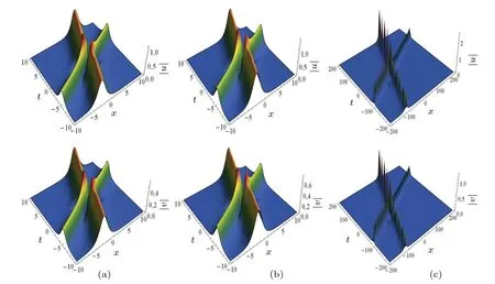
Fig.1.Two-soliton interaction diagram via solutions(16),with k1=1+0.2i,k2=0.6+i,α1=n1=1,n2=1/2,m1=2,but(a)with σ1=2,σ2=2,(b)with σ1=2,σ2=?2,(c)with k1=0.08+0.2i,k2=0.08+i,σ1=?2,σ2=?2.

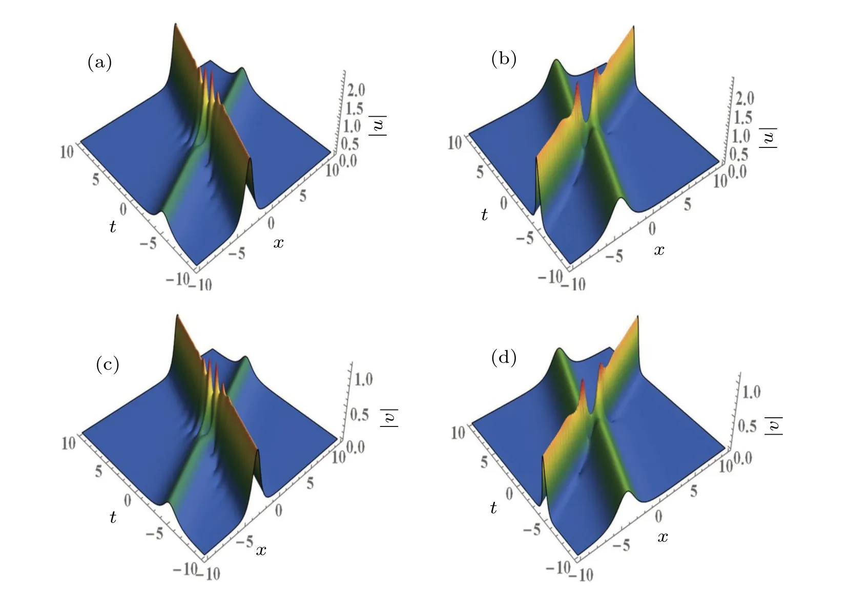
Fig.2.Two-soliton interaction diagram shown in solutions(16)with the same parameters as in Fig.1(a),but[(a),(c)]with k1=2+0.2i and[(b),(d)]with k2=?2+i.

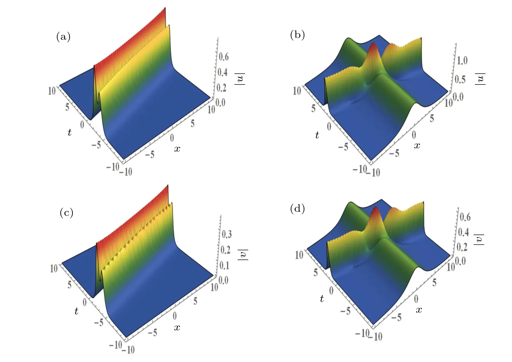
Fig.3.Two-soliton interaction diagram in solutions(16)with the same parameters as in Fig.1(a),but[(a),(c)]with k1=1+2i,k2=0.6+2i,and[(b),(d)]with k1=1?2i,k2=0.6.

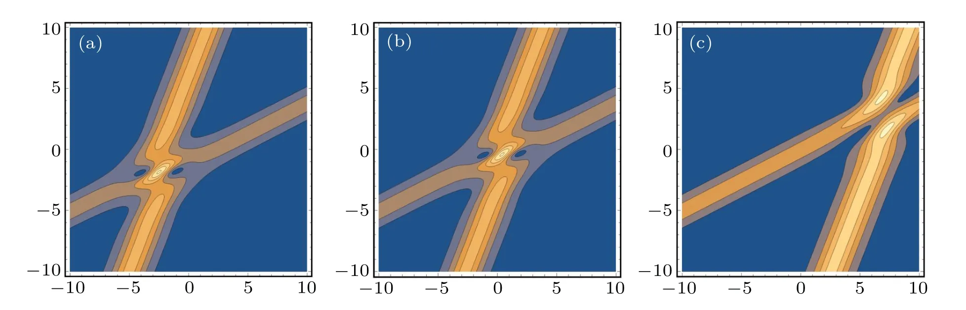
Fig.4.The contour plot of the absolute value of the function u in expression(16)with the same parameters as given in Fig.1(a),but(a)with n1=?10,n2=0.5,(b)with n1=?1,n2=0.5,and(c)with n1=0.005,n2=0.5.

Figure 4 shows the contour plot of the absolute value of the functionuin expression (16) with the same parameters as given in Fig.1(a), but Fig.4(a) withn1=?10,n2=0.5,Fig.4(b) withn1=?1,n2=0.5, Fig.4(c) withn1=0.005,n2=0.5.We find that the absolute value of the ration1/n2affects the location of the collision of two solitons,where the energies of the two solitons converge.Fixingn2and decreasing the absolute value ofn1,we find that one of the two-soliton shifts to the right,and the other one does not shift;the change of the contour plot of the absolute value of the functionvin expression (16) is the same as the functionu.When the absolute value of the ration1/n2decreases, the location of the collision of two solitons moves to right upper the coordinate surface.In addition,the value ofm1has a similar effect on the ration1/n2.

4.2.Discussion of the three-soliton solutions

Figure 5 portrays the interaction diagram of three-soliton solutions with the parametersk1=0.6+0.2i,k2=0.6+i,k3=0.6?0.5i,α1=?=n1=n2=n3=1,σ1=σ2=?2.By observing Fig.5, the three-soliton solutions for Eq.(4),which reads the Manakov model of all-defocusing type, we can find that the all-defocusing type Manakov model admits bright-bright-bright solitons solutions.This conclusion can be regarded as a generalization of the two-soliton case.A graph of|u|is shown in Fig.5(a),where the collision causes the amplitude of one soliton to be suppressed and the amplitude of the other two solitons to be enhanced.It is interesting to note that the graph of|v| shown in Fig.5(b) also shows the same kinds of changes.The similar phenomena of this form of intensity redistribution have surfaced in the potential application to communication signal amplification.[18]

Figure 6 portrays the interaction diagram of three-soliton solutions (20) with the parametersσ1= 2,σ2= 2,α1=?=n1=n2=n3= 1,k3= 1.2?0.5i, but Fig.6(a) withk1=1+0.2i,k2=0.6+i, Fig.6(b) withk1=2.5+0.2i,k2=0.6+i,Fig.6(c)withk1=1+0.2i,k2=2.5+i.By observing the three-soliton solutions shown in Figs.6(a)–6(c),in comparisons of the real parts of wave numbersk1andk2shown in Figs.6(a)and 6(b),Figs.6(a)and 6(c),it can be found that the amplitudes of the solitons increase with the absolute value of the real parts ofkj(j=1,2), the result is the same as the case of two solitons.It means that the wave amplitude of the three-soliton solution is also controlled by the wave number of the real parts ofkj.

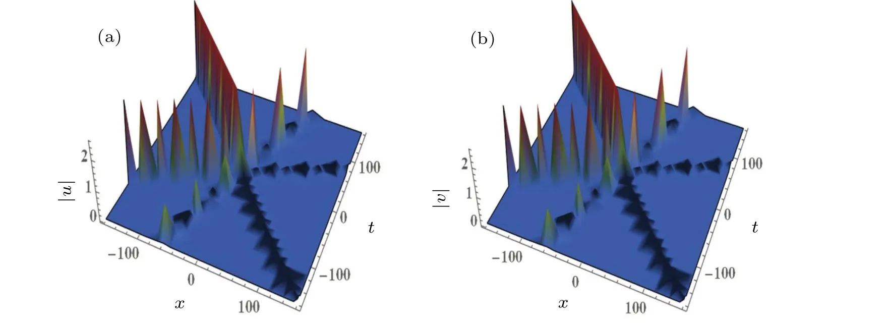
Fig.5.Three-soliton interaction diagram via solutions(20),with k1 =0.6+0.2i,k2 =0.6+i,k3 =0.6 ?0.5i,α1 =? =n1 =n2 =n3 =1,σ1=σ2=?2.

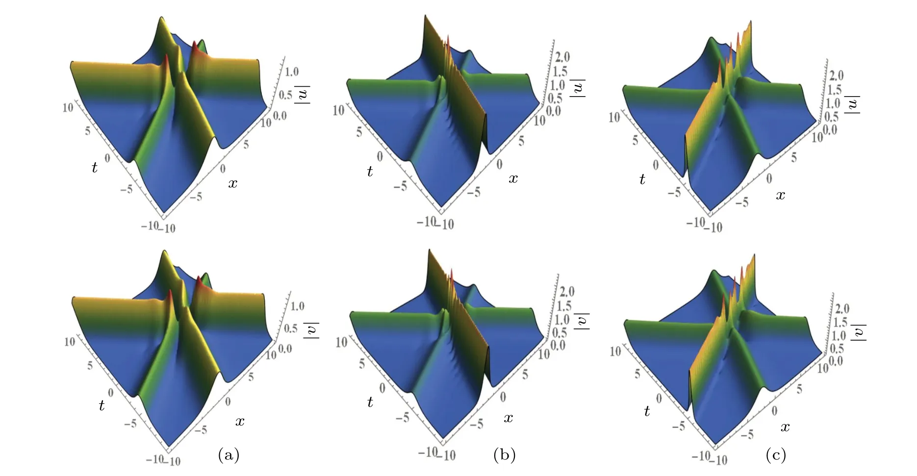
Fig.6.Three-soliton interaction diagram via solutions (20), for σ1 =2, σ2 =2, α1 =? =n1 =n2 =n3 =1, k3 =1.2 ?0.5i: (a) with k1=1+0.2i,k2=0.6+i,(b)with k1=2.5+0.2i,k2=0.6+i,(c)with k1=1+0.2i,k2=2.5+i.

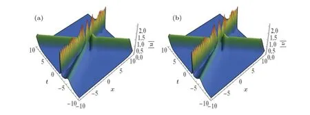
Fig.7.Three-soliton interaction diagram in solutions(20)with the same parameters as given in Fig.6(b),but with k1=2.5+2.5i.

When the imaginary parts of one wave numberkj(j=1,2,3) are changed and the other parameters remain unchanged, we can control the wave to rotate.This means that the propagation directions of solitons are determined by the imaginary parts ofkj(j=1,2,3).Compared Fig.6(b) and Fig.7,when we change the imaginary part of the wave numberk1,from 0.6 to 2.5,the imaginary part value ofk1is greater than zero,the soliton’s propagation path forms an acute angle with the positivex-axis,the angle decreases with the increase of the imaginary part ofk1, and the other laws in the case of two solitons are also true.

Figure 8 portrays the interaction diagram of three-soliton solutions(20)with the parametersk1=1+0.2i,k2=0.6+i,k3=1.2?0.5i,α1=?=1,σ1=2,σ2=2,but Fig.8(a)withn1=n2=n3=1,Fig.8(b)withn1=n3=1,n2=0.01,and Fig.8(c) withn1=n3=1,n2=100.In Figs.8(a)–8(c), we fixn1=n3=1 and change the absolute value ofn2,and it is found that one of the three solitons shifts and the other two solitons do not shift.In comparison of Figs.8(a)and 8(b),one of the three solitons shifts to the right with decrease of the absolute value ofn2.In comparison of Figs.8(a)and 8(c),one of the three solitons shifts to the left with increase of the absolute value ofn2.The change of the functionvin expression(20)is the same as the functionu.We can see that the value of the rationi/njaffects the location of the collision of three solitons,and the law is also the same as in the case of two solitons.

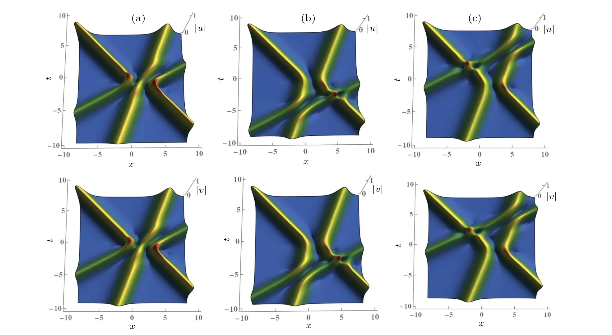
Fig.8.Three-soliton interaction diagram of solutions(20),for k1 =1+0.2i,k2 =0.6+i,k3 =1.2 ?0.5i,α1 =? =1,σ1 =2,σ2 =2: (a)with n1=n2=n3=1,(b)with n1=n3=1,n2=0.01,and(c)with n1=n3=1,n2=100.

5.Conclusions

In summary, we have studied a coupled Schr¨odinger equation that comes from the Boussinesq equation of atmospheric gravity waves by using multiscale analysis and reduced perturbation method to describe Rossby waves.By setting values of parameters, we obtain the Manakov model of all-focusing, all-defocusing and mixed types, and utilize the Hirota bilinear method to give the two-soliton and threesoliton solutions.We find that the all-defocusing type Manakov model admits bright-bright soliton solutions.This finding has not been reported in the literature to our best knownledge.We also find that the all-defocusing type Manakov model admits bright-bright-bright soliton solutions,which can be regarded as a generalization of the two-soliton solutions.

Then,we discuss the influence of free parameters on the wave amplitude,the propagation direction and the location of the collision in the two-soliton and three-soliton solutions for the all-focusing type Manakov model.The following conclusions are drawn:

(i)The amplitudes of the solitons increase with the absolute value of the real parts ofkj(j=1,2,3)for the two-soliton and the three-soliton solutions.

(ii) The propagation direction of solitons can be controlled by the imaginary part ofkj(j=1,2,3) for the twosoliton and the three-soliton solutions.

(iii)The absolute value of the ration1/n2changes the location of the collision in the two-soliton and three-soliton solutions.

Solitons maintain their original amplitudes, velocities,and shapes in elastic collisions, with the exception of a little phase shift following the collision.[44]From this point of view,the collisions in Figs.1(a), 1(b), 2, 3, 6, 7, and 8 are elastic,and the collisions in Figs.1(c)and 5 are inelastic.

It is crucial to keep in mind that the Hirota bilinear method does not work whengn(x,t) =hn(x,t) =fn(x,t) =0, (n= 5,6,...) [orgn(x,t) =hn(x,t) =fn(x,t) = 0, (n=7,8,...)] are not zero in the case of solving two-soliton (or three-soliton) solutions.The result shows that the soliton propagation for the coupled Schr¨odinger equation describing Rossby waves we studied is affected by the above factors but may not limited to them.There should be more cases necessarily to be investigated.Whether the intensity redistribution phenomena we observed in Fig.5 can occur in otherNsoliton cases requires further investigation.We will investigate whetherN-soliton solutions have similar properties in another work.These conclusions are useful for setting a simulation scene in research of Rossby waves.

Acknowledgements

This work was supported by the National Natural Science Foundation of China (Grant Nos.12102205 and 12161065),the Scientific Research Ability of Youth Teachers of Inner Mongolia Agricultural University(Grant Nos.JC2021001 and BR220126),the Natural Science Foundation of Inner Mongolia Autonomous Region of China(Grant No.2022QN01003),and the Research Program of Inner Mongolia Autonomous Region Education Department(Grant Nos.NJYT23099 and NMGIRT2208).