Structure of continuous matrix product operator for transverse field Ising model: An analytic and numerical study

Yueshui Zhang(張越水) and Lei Wang(王磊)

1Institute of Physics,Chinese Academy of Sciences,Beijing 100190,China

2University of Chinese Academy of Sciences,Beijing 100049,China

3Beijing National Laboratory for Condensed Matter Physics and Institute of Physics,Chinese Academy of Sciences,Beijing 100190,China

4Songshan Lake Materials Laboratory,Dongguan 523808,China

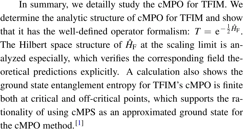
We study the structure of the continuous matrix product operator (cMPO)[1] for the transverse field Ising model(TFIM).We prove TFIM’s cMPO is solvable and has the form. ?HF is a non-local free fermionic Hamiltonian on a ring with circumference β, whose ground state is gapped and non-degenerate even at the critical point. The full spectrum of ?HF is determined analytically. At the critical point,our results verify the state–operator-correspondence[2] in the conformal field theory(CFT).We also design a numerical algorithm based on Bloch state ansatz to calculate the lowlying excited states of general(Hermitian)cMPO.Our numerical calculations coincide with the analytic results of TFIM.In the end,we give a short discussion about the entanglement entropy of cMPO’s ground state.

Keywords: continuous matrix product operator,transverse field Ising model,state–operator-correspondence

1. Introduction

Tensor network approaching thermal states has a long history. Back in the age of the density matrix renormalization group, the transfer matrix renormalization group[3]based on Trotter decomposition has been developed to calculate thermodynamic quantities of low-dimensional strongly correlated systems. Recently, a new tensor structure named continuous matrix product operator (cMPO)[1]has been developed. Different from previous methods, cMPO eliminates imaginarytime discretization error.

Before going to the theme,we should give a brief review of cMPO to familiarize readers with the relevant notations and more importantly,to show the mechanism behind cMPO.For simplicity,we consider a Hamiltonian with nearest interaction(although in general,cMPO method is suitable for more complex interactions,even for long-range interactions[1])

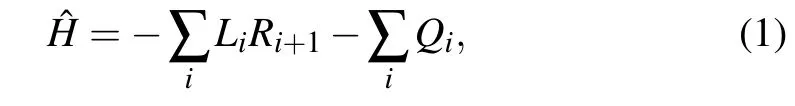
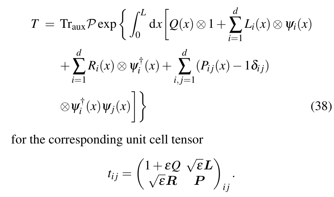
whereiis the label of lattice site.Qi,Li,andRiare local operators living on the Hilbert space of the single sitei. Considering the evolution operator e-τ?H,the first-order approximation 1-τ?Hcan be represented as a matrix product operator(MPO)whose unit cell is an infinitesimal tensor parameterized byτ,as shown in Figs.1(a)and 1(b),

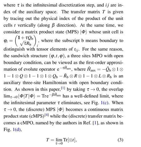
which can be viewed as a continuous transfer matrix without discretization error. The corresponding partition function is the product of cMPO:Z=Tr[TL], if we assume the system hasLsites. In the thermodynamic limitL →∞, the free energy per sitefis determined by the dominate eigenvalueΛ0of cMPO:β f=-lnΛ0.

In cMPO’s framework, the key point is, under the assumption the dominate eigenstate|Φ〉(we name it the ground state in the following) of transfer matrixTcan be approximated by a matrix product state (MPS) in some sense, when taking discretization stepτto be zero, the overlap〈Φ|T|Φ〉is well-defined and at the same time the ground state|Φ〉is parameterized as a cMPS,as we have explained above.

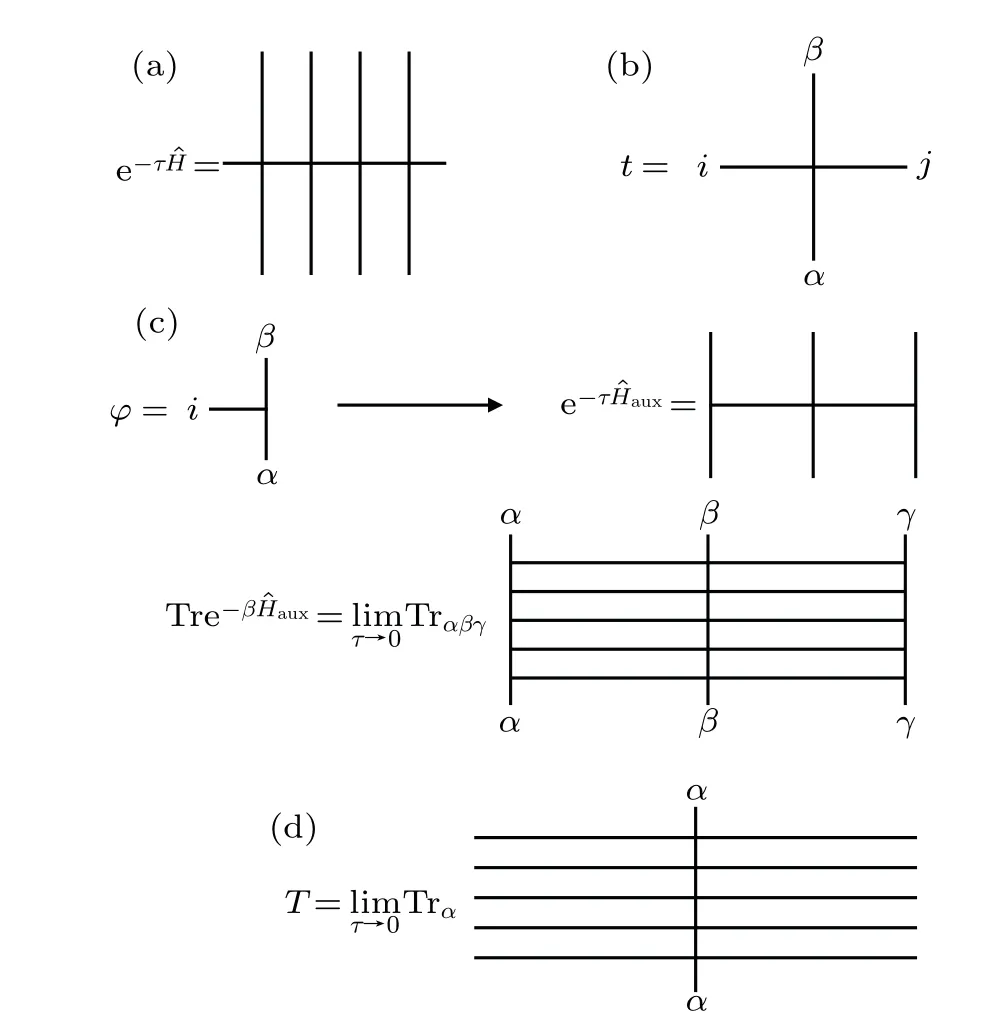
Fig.1. The graphic representation of cMPO.(a)The unit cell of cMPO can be constructed from the corresponding infinitesimal evolution operator e-τ ?H. (b)The graphic representation of cMPO’s unit cell tensor t,where{i j}is the virtual index,while{αβ}is the physical index.(c)By introducing a cMPS|Φ〉with unit cell tensor φ,the sandwich structure〈Φ|T|Φ〉is well-defined when τ →0 in cMPO method. The auxiliary hHamiltonian ?Haux is independent of τ. (d)cMPO is a transfer matrix by taking τ →0 if the continuum limit truly exists.

However,strictly speaking,although the existence of the overlap〈Φ|T|Φ〉at continuum limitτ →0 is enough for numerical calculation in cMPO method, the existence of cMPOTat the operator level as the continuum limit of certain(discrete)MPO,which has been defined in Eq.(3),remains to be verified. In another word, we could ask whether the transfer matrixTis a well-defined(continuous)operator when taking discretization error to be zero? As we have pointed out in the last paragraph,cMPO seems to be an intermediate notation in practical calculation: if we assume|Φ〉is a cMPS, then the overlap〈Φ|T|Φ〉is well-defined,no matter whetherTcan exist individually as an operator or not when discretization stepτto be zero.

We leave the tedious technical details in the Appendix.In Appendix A, we review the diagonalization procedure of the transfer matrix for arbitrary trotter stepτ. In Appendix B,we show how to take the continuum limit to get the operator formalism of TFIM’s cMPO.In Appendix C,we show the detailed calculation of the correlation matrix and the corresponding integral equation as its continuum limit. In Appendix D,we give the analytic expressions of the ground state’s correlations at the continuum limit for TFIM’s cMPO.In Appendix E,we prove at classical Ising limith=0, cMPO’s ground state has a simple cMPS representation. In Appendix F,we explain the explicit tensor constructions for our numerical algorithm.

2. Operator formalism of cMPO

The Hamiltonian of the 1D transverse field Ising model is

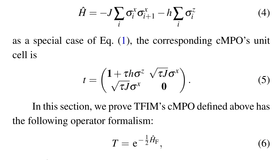
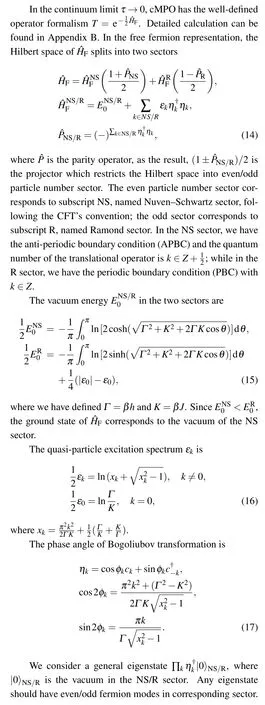
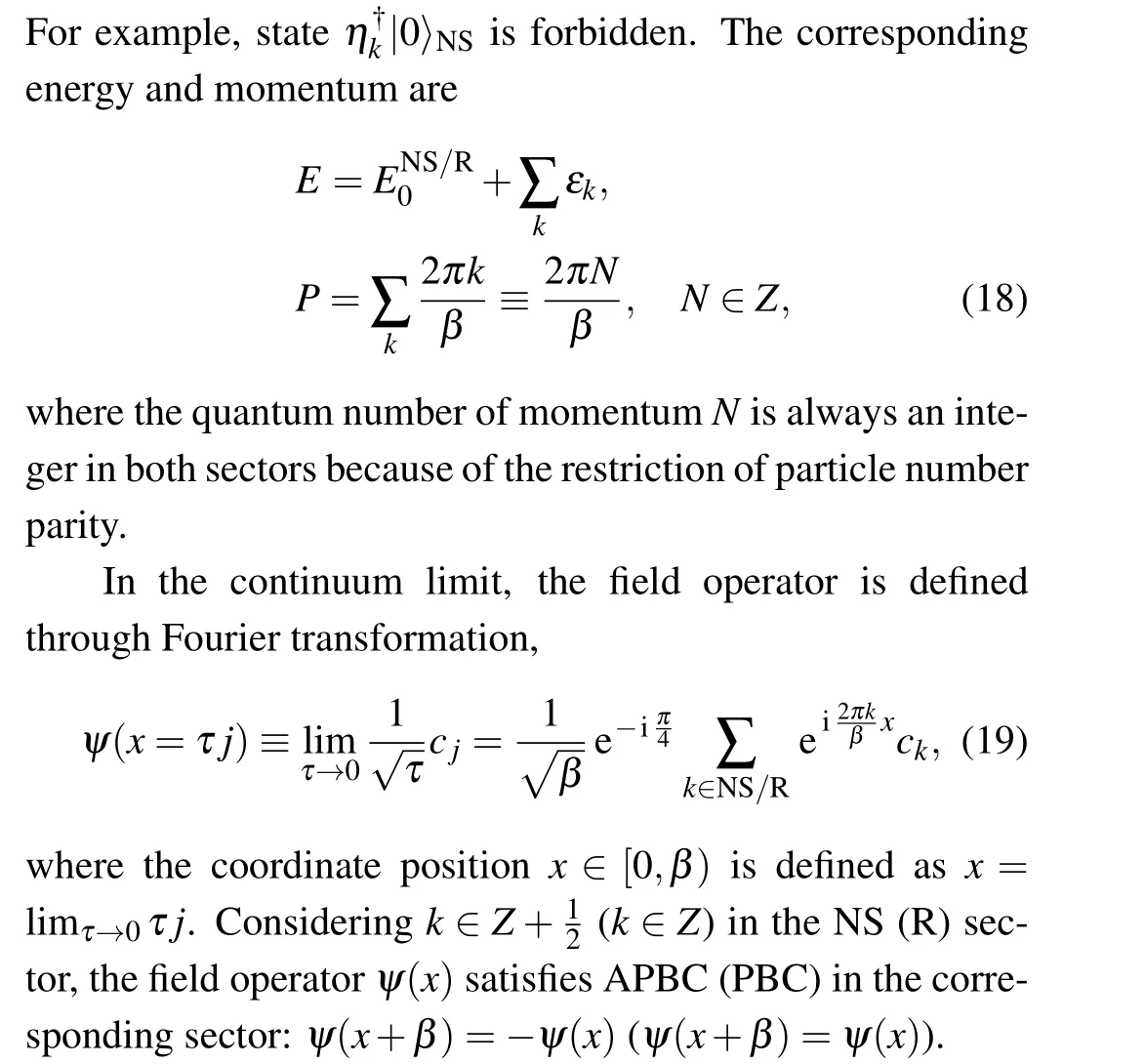
where ?HFis a free fermionic Hamiltonian living on a ring of lengthβ. ?HFis diagonal in{ηk}representation, which is the momentum space representation following a Bogoliubov transformation. The explicit expression of ?HFis given in Eq.(14). The corresponding spectrum and Bogoliubov angle are given in Eqs. (15)–(17). We can use Eq. (19) to find the coordinate space representation of ?HF, which is a non-local QFT.

We prove Eq.(6)in two steps. In the first step,we solve the transfer matrixTunder arbitrary trotter stepτ. In the second step,we takeτto be zero to find the continuum limit ofT.While in the first step,an important trick is employed: instead of usingtin Eq.(5),we can use ?tin Eq.(11)as the unit cell of cMPO,since ?tandtare the same infinitesimal tensor up to the first order ofτ: ?t=t+O(τ2). Whenτ →0,T=Tr[?t]and ?T=Tr[??t]will correspond to the same cMPO,if the continuum limit truly exists.

We divide this section into two parts. In part I, we construct ?t, which is the same infinitesimal tensor astwhenτ →0, from the MPO representation of infinitesimal evolution operator e-τ?Hand prove the solvability of transfer matrix ?T=Tr[??t]at arbitrary trotter stepτ. In part II, we show the operator formalism of cMPOTtruly exists at the continuum limit and give its explicit form analytically.

2.1. Solvability at arbitrary trotter step τ

2.1.1. construct unit cell ?t

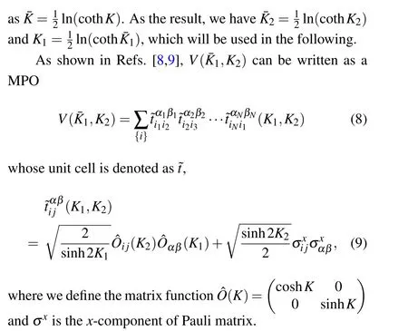
Motivated by the paper,[8]we consider the second order trotter approximation e-τ?H=V(ˉK1,K2)+O(τ3),with

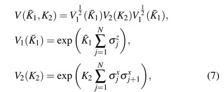
where the trotter stepτis defined byβ=Nτ, and ˉK1=τh,K2=τJ. The functional relation betweenKand ˉKis defined

Whenτ →0, using Taylor expansion aboutτ, we find tensor ?tcoincides withtup to the first order ofτ,

Since ?tandtare the same infinitesimal tensor,TFIM’s cMPO can be rewritten as ?T=limτ→0Tr[??t].

2.1.2. Map ?T to be free fermion

The solvability of ?Tis based on the following algebraic identity:[8]

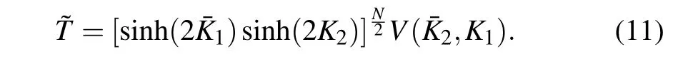
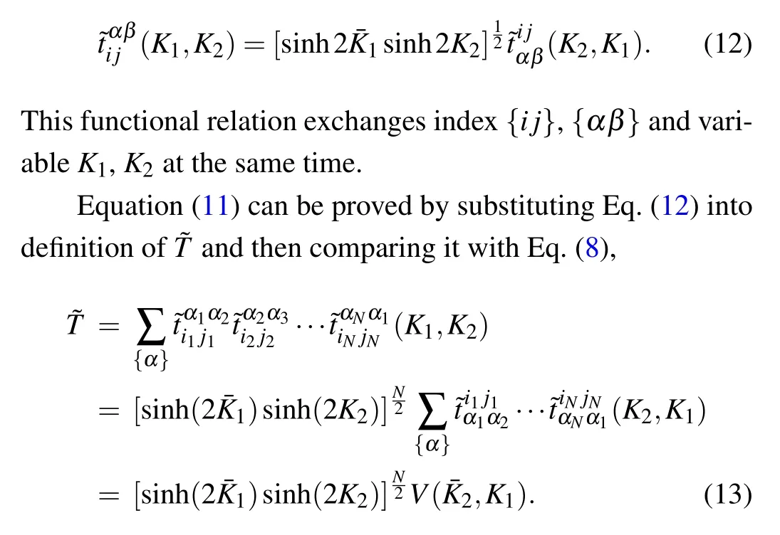
In Eq.(11), ?Tis factorized into operatorV(ˉK2,K1)and a scalar factor. SinceV(ˉK2,K1)is also the transfer matrix of the two-dimensional Ising model,[10]V(ˉK2,K1),and ?Tat the same time,can be mapped to free fermion and exactly solvable.

To prove Eq. (11), we need the following dual relation,which can be easily checked from Eq.(9),

Technical details about the diagonalization ofV(ˉK2,K1)can be found in the classic paper[10]or Appendix A.

2.2. Operator formalism at the continuum limit

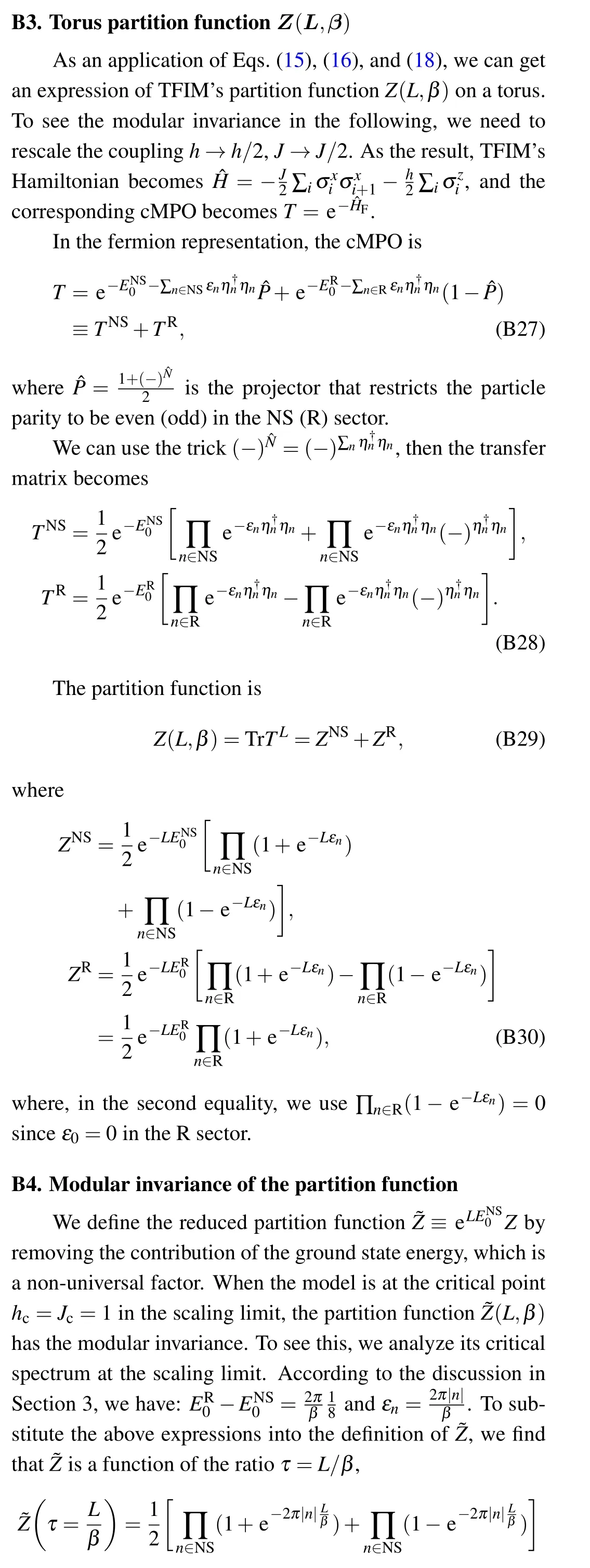
We can also use Eqs. (15) and (16) to calculate the partition functionZ(L,β) on a torus. Furthermore, to compare with the formula calculated by diagonalization of the physical Hamiltonian, we can explicitly verify the modular invariance of Ising CFT for critical TFIM in the scaling limit. A calculation can be found in Appendix B.

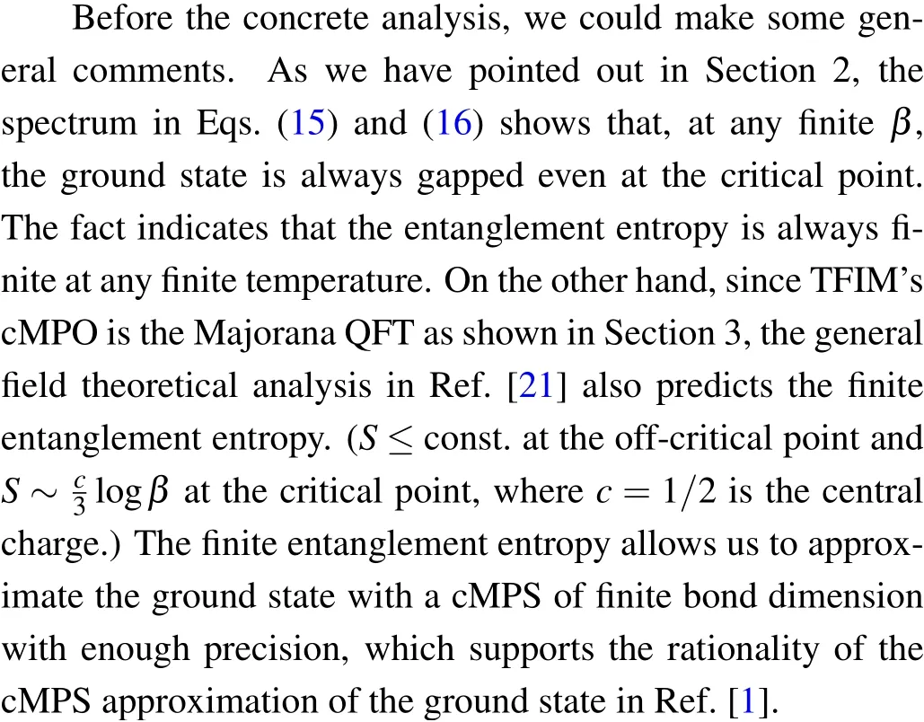
Finally, we should point out that, the spectrum in Eqs. (15) and (16) suggests that, for any finiteβ, even at the critical pointJ=h, there always exists a finite energy gap of order 1/β,which indicates the finite entanglement entropy of the ground state.

3. Hamiltonian structure at the scaling limit

We divide this section into two parts. In the first subsection,we show that the Hamiltonian ?HFis equivalent to the familiar free Majorana QFT at the scaling limit. Although,in general, the Hamiltonian is non-local as explained in Section 2. In the second subsection,we verify the state–operatorcorrespondence from the Hamiltonian structure explicitly.

3.1. Map to Majorana QFT

In the scaling limit,the short-distance feature washes out.We only care about the behavior at the low-energy scale of order 1/βcorresponding to the long-wavelength limit. We can expand the excitation spectrum and phase angle in Eqs. (16)and(17)atβ →∞to the first order of 1/β,

It is well-known that the effective theory of TFIM is the Majorana QFT. We find the Hamiltonian ?HFof cMPO in Eq.(22)is also the Majorana QFT.This fact reflects the rotation symmetry of Euclidean field theory.

3.2. State–operator-correspondence at m=0

Whenm= 0, ?HFis critical and restores the conformal symmetry, which can be described by Ising CFT on a cylinder.[13,14]

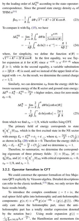
In the cMPO’s framework, we exchange the space and time, where we viewβas space while the time direction is discrete and labeled by the index of lattice sitei. Because of the discretion of time, the continuous evolution operator becomes the discrete cMPO:T= e-λ?HF, whereλis some non-universal normalization factor. In the TFIM case,we will seeλ=1/2 in the following as already shown in Eq.(6). To see the conformal structure of cMPO, we first determine the central chargecand critical exponentxσfrom vacuum energy shift in Eq.(15),where the identity corresponds to ground state|0〉NSand the spin operator corresponds to zero mode state in the R sectorη?0|0〉R(Remember in R sector,only odd particle number state is allowed). We will also show the energy operator corresponds to the first excited state in the NS sector.Furthermore, since the operator formalism of the free Majorana field in Eq. (22) (withm=0) is well known,[13,14]the entire conformal tower structure is obvious. Using transformation relation Eq. (19), we can build a dictionary between fermion representation in Eq.(14)and CFT’s operator formalism explicitly.

3.2.1. Determine c and xσ from vacuum energy shift

Using the transformation relation between{ηn}and{bn},we list the one-to-one map between the fermion representation in Eq.(14)and CFT’s operator formalism in Eq.(26)in a dictionary.

Structure of Hilbert space of ?HF Primary states: Fermion Virasoro|pˉp〉,xp=p+ ˉp representation algebra|1〉≡|0ˉ0〉 |0〉NS |0〉NS|ε〉≡|1 2 ˉ1 2|0〉NS|σ〉≡| 1 2〉 η?12η?-1 2ˉb-12|0〉NS b-1 16 ˉ1 16〉 η?0|0〉R (ˉb0-ib0)|0〉R Other ∏{k}η?k|0〉NS/R ∏{n},{ˉn}L-nL-ˉn|pˉp〉excited #{k}=even in NS; n,ˉn ∈Z+,states #{k}=odd in R |pˉp〉∈{|1〉,|ε〉,|σ〉}Energy E=∑εk E= 2π β (xp+∑n+∑ˉn)Momentum P= π β ∑k P= 2π β (∑n-∑ˉn)

Additionally, according to the above analysis, to make ?HF±?Pbe holomorphic (anti-holomorphic) in Eq. (26), the non-universal factorλshould be 1/2 in TFIM’s cMPO as shown in Eq.(6).

4. Numerical algorithm for excitation

Motivated by the analytic results of TFIM’s cMPO and field theoretical prediction of CFT, which has been detailed discussed in previous sections, in this section, we show how to numerically calculate the low-lying excited states of cMPO for the general lattice model (with the assumption the corresponding cMPO is Hermitian)and extract critical information from numerical data. (In history,there already exist some numerical works to verify the state–operator-correspondence by studying the low-lying excited states of the lattice Hamiltonian ?Hlatt.[15–17])

We first briefly review the variational cMPS method for cMPO’s ground state search, which has a detailed discussion in the original paper for the cMPO method.[1]Next, we explain the method for excited states’ calculation based on the Bloch state ansatz. Finally,we show the numerical results for TFIM’s cMPO as a benchmark.

4.1. The cMPS ansatz for ground state

4.2. Bloch state ansatz for excited state

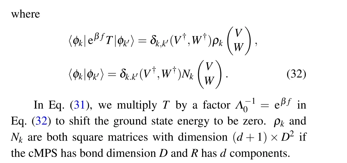
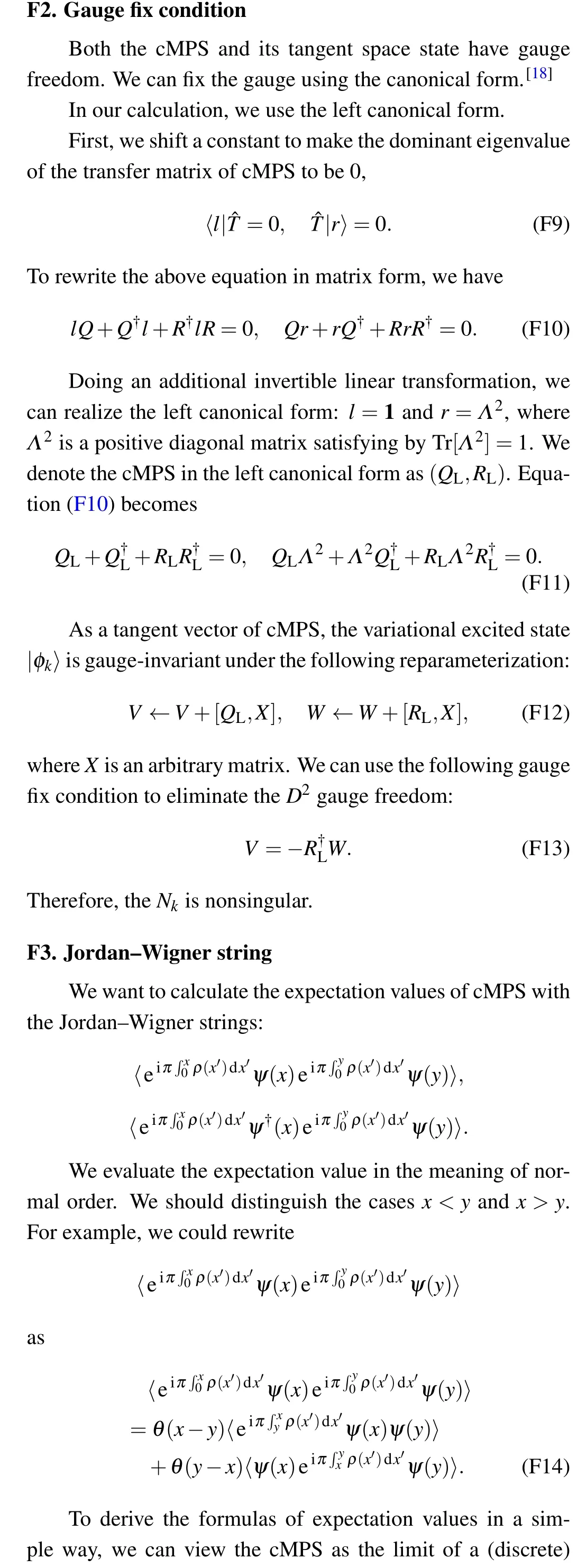
However, technically,Nkis singular because of gauge freedom. To resolve the problem, we can fix the gauge to reduce the parameter space’s dimension to bed×D2and thus makeNkbe full rank.[18]Under the gauge fixing,the solution of the above eigen-equation Eq.(31)gives thedD2lowest excited states parameterized by{Vn,Wn}with the corresponding excitation energies{ΔEn},n ∈1,2,...,dD2. The explicit expressions ofρkandNkcan be found in Appendix F.

4.3. Benchmark for TFIM

4.3.1. Excitation at the critical point

To test our algorithm for excitation,we show the numerical results of TFIM’s cMPO at the critical pointhc=Jc=1.

Fig.2. (a)The first three excitations spectrum as function of β in P=0 sector, where the ground state energy is set to be zero. The curves are analytic results and points are numerical data.The lowest spectrum corresponds to the primary field of spin ΔER0; the second spectrum corresponds to the primary field of energy ΔEε.(b)The first three excitations spectrum as the functions of β in P=1 sector.

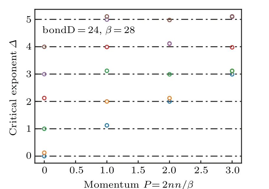
Fig.3. Structure of conformal tower for TFIM’s cMPO at β =28. The variational cMPS has bond dimension bondD=24.

We first verify the formulas of spectrum in Eqs.(15)and(16). We plot the excitation spectrum as the function ofβin the momentum sectorsP=0 andP=1, as shown in Fig. 2,

where the curves are analytic results and the points are numerical data.

We can also verify the conformal data of Ising CFT atβ ?1. In Fig.3,we plot the low-lying excitation spectrum atβ=28, which has the structure of conformal tower of Ising CFT,agreeing with the analytic calculation in Section 3. Using finite size scaling, at the numerical level, we confirm the central chargec=1/2 and critical exponents for three primary fieldsx1=0,xσ=1/8 andxε=1 in Fig.4.

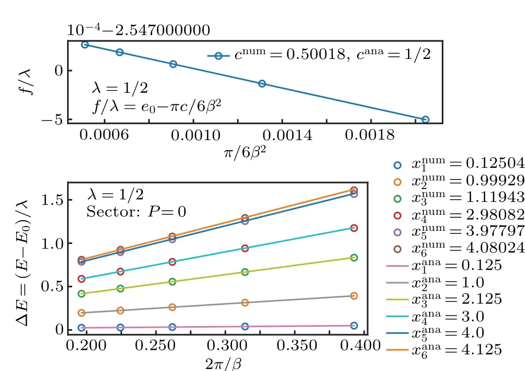
Fig. 4. (a) The central charge c=1/2 from finite size scaling of the free energy. (b) The critical exponents from finite size scaling of the excitation spectrum. The superscript‘num’ means numerical data and‘ana’means analytic results. The first two exponents correspond to spin and energy: x1 ≡xσ,x2 ≡xε. The identity is trivial,which is set to be zero. The λ =1/2 is the non-universal factor in Eq.(6).

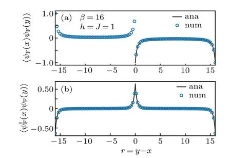
Fig. 5. Two-point correlation functions of the ground state of TFIM’s cMPO.The curves are analytic solutions while the points are numerical results. We choose parameters β =16, h=J =1. The cMPS’s bond dimension is bondD=16. (a)〈ψF(x)ψF(y)〉and(b)〈ψ?F(x)ψF(y)〉.

4.3.2. Correlation for ground state

To finish this subsection, we also comment to explain why the underlying fieldψ(x) of cMPS is bosonic. Since we could view the cMPO as the continuum limit of a discrete spin model, when we take the continuum limit, the local spin (hard-core boson) operatorσ+jcorresponds to the

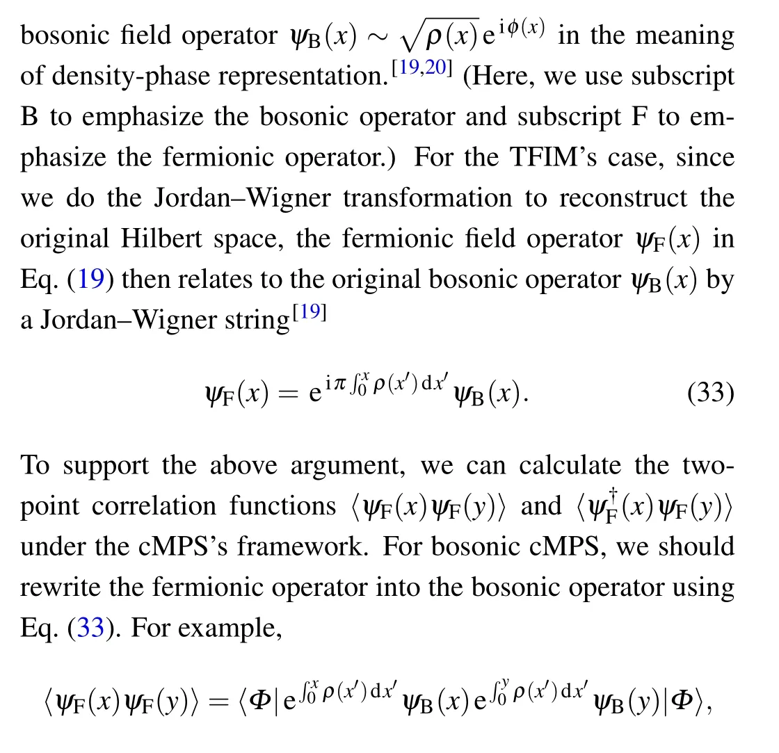
where|Φ〉is the variational cMPS ground state in Eq. (27).We compare the numerical results with the analytic results in Fig.5,which coincides with our prediction. Additionally,results in Fig.5 also show that the variational cMPS ground state truly captures the exact ground state of TFIM’s cMPO,which is a fermionic Gaussian state and thus is completely captured by its two-point correlations.

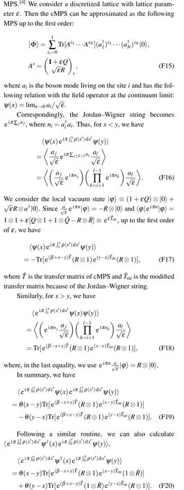
The analytic expressions of the fermionic correlation functions can be found in Eqs.(D2)and(D3)in Appendix D.The technical details of calculating cMPS’s expectation values about operators with a Jordan–Wigner string have been explained in Appendix F.

5. Entanglement entropy

In this section,we discuss the ground state entanglement entropy of cMPO based on the analysis of TFIM.

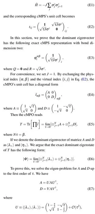
Although we cannot find the exact cMPS representation of the ground state for TFIM’s cMPO,at the limit caseh=0,the ground state is a simple cMPS with bond dimension two,see Appendix E,

Its entanglement entropy is independent of the subsystem’s sizeβ′as shown in Eq.(E16):S=ln2+δS(β),which tends to beS=ln2 whenβ →∞. The correction termδS(β)～e-2β(1-2ln2)＜0 is exponential small. (We set the coupling constant to beJ=1 by absorbingJintoβ).

In the following, we first verify the finite entanglement entropy for TFIM by diagonalizing the subsystem’s correlation matrix under a small trotter step[6,7]in the first subsection.We also give an integral equation as the continuum limit of the correlation matrix in the second subsection.

5.1. Entanglement entropy for TFIM:numerical results

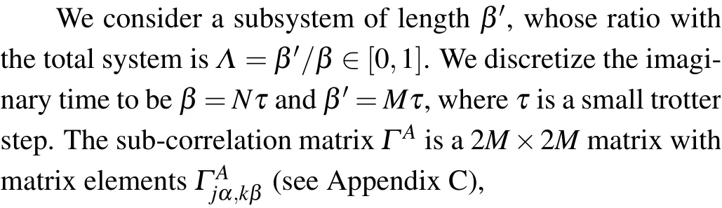
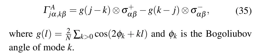
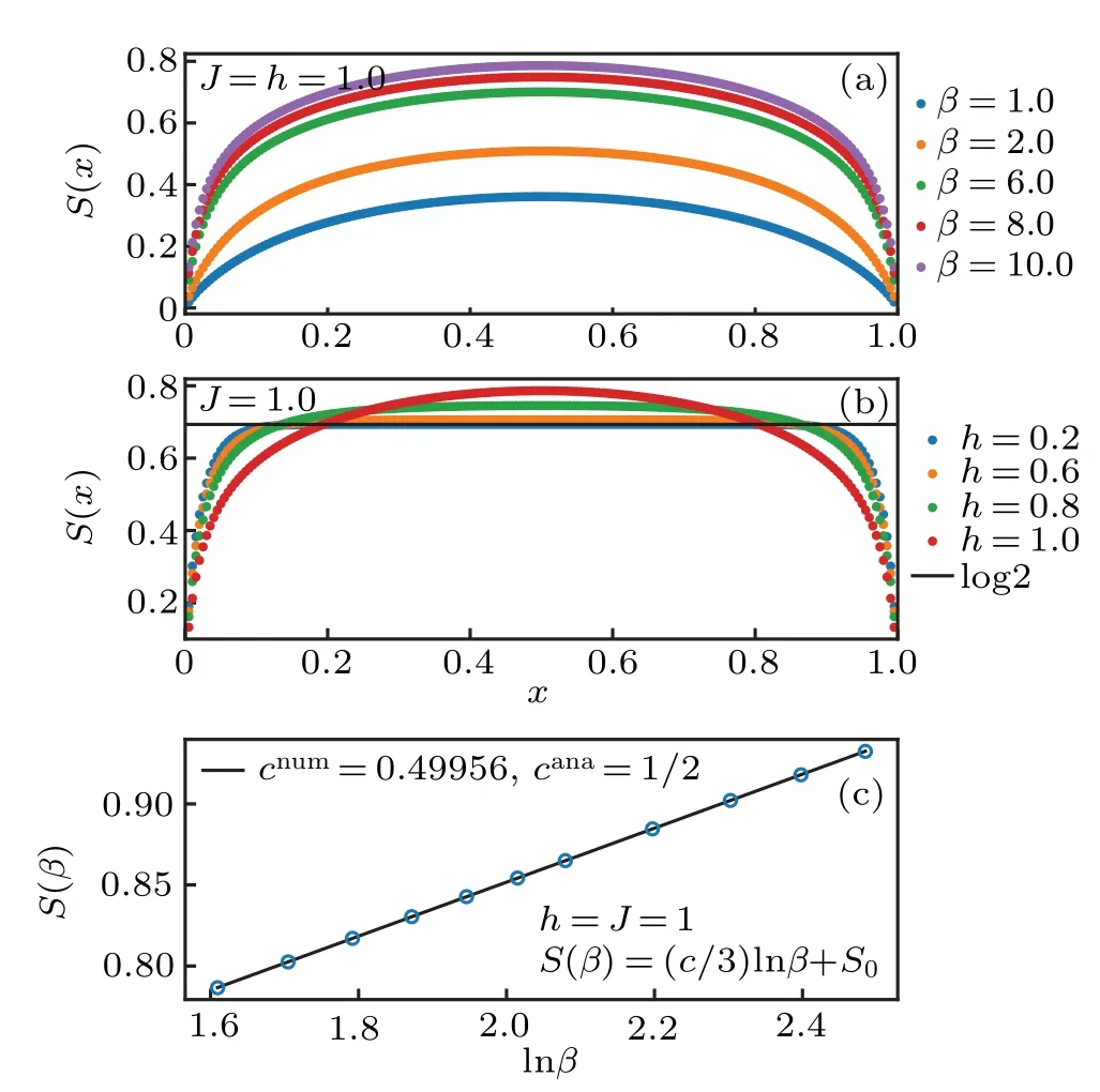
Fig.6. (a)The critical entanglement entropy with h=J=1 for different β. (b) The off-critical entanglement entropy at β =10, which has a lower bound S=ln2. The x-axis labels the ratio x=β′/β, where β′ is the subsystem’s size. (c)The critical entanglement entropy as the function of β. We verify the central charge c=1/2 from the scaling of the critical entanglement entropy.

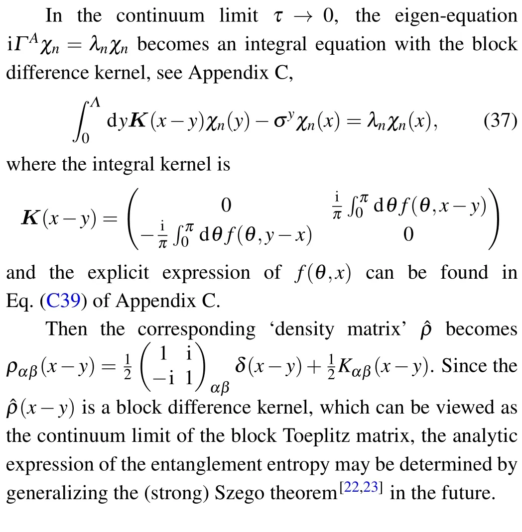
5.2. Integral equation for correlation matrix

6. Conclusions and outlook

Motivated by the Hamiltonian structure of TFIM’s cMPO and the theoretical predictions of CFT,we also design an algorithm to calculate the critical exponents for the general lattice model through the excitation spectrum of the corresponding cMPO.We use the analytic results of TFIM as the benchmark.Our numerical algorithm may also be used to calculate the excited states for the continuous model on a ring.

Although the solvability of TFIM’s cMPO is heavily on the special structure of the two-dimensional Ising model, we tend to believe that the Hamiltonian structure for cMPO is universal to some extent. In fact, in the bethe ansatz techniques for thermodynamics, apart form the traditional Yang–Yang approach,[24]there also exists the quantum transfer matrix approach,[25,26]which may be viewed as the (integrable)cMPO in some sense.

The derivation in this work is based on taking the continuum limit of a certain lattice model.However,it is not difficult to show that the cMPO has a very similar(lattice independent)integral formalism to the cMPS case,

It is also possible to construct a series of solvable models sharing the same ground states with the corresponding cMPOs,whose ground states have the cMPS structure. Detailed analysis will appear in the late.

Appendix A:Diagonalization ofV

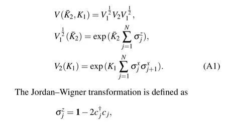
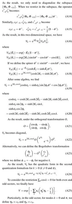
In this section, for the reader’s convenience, we review the procedure of the diagonalization of the transfer matrixVin Eq.(7),following the classic paper,[10]where the slight difference is the exchange ofV1andV2in our definition. We map the transfer matrix to the free fermion and then diagonalize it using the Bogoliubov transformation.

For simplicity,we define 1=β=Nτand letNbe even.We need to diagonalize the following transfer matrix:

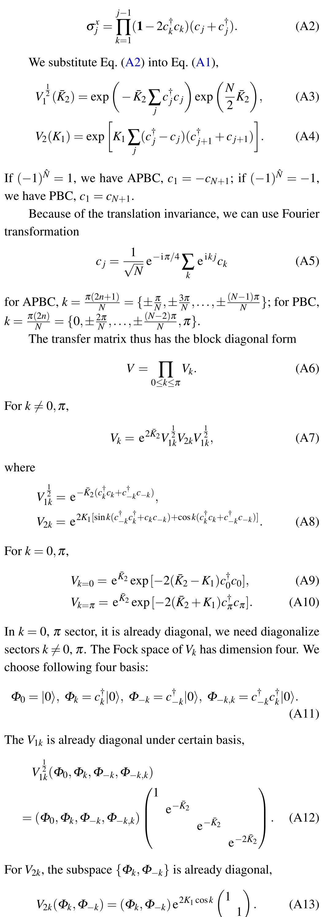
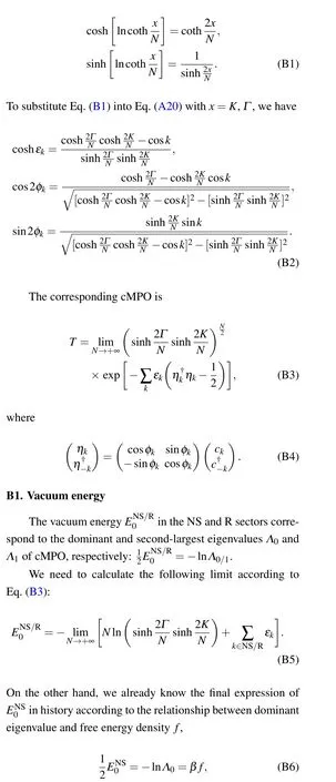
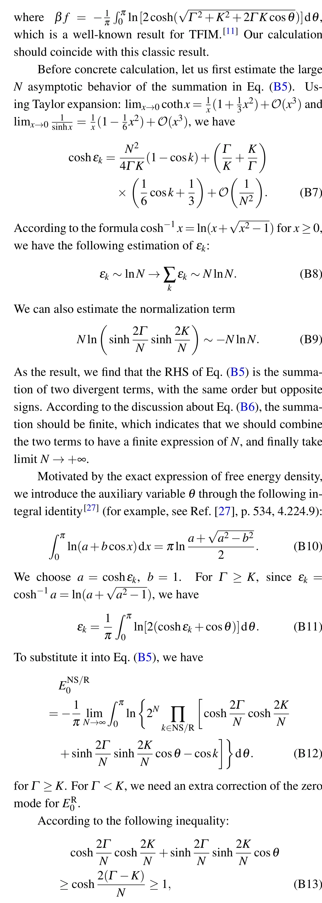
Appendix B:Spectrum at the continuum limit

We first summarize the above formulas using parametersKandΓ. The following identity proves to be useful:k

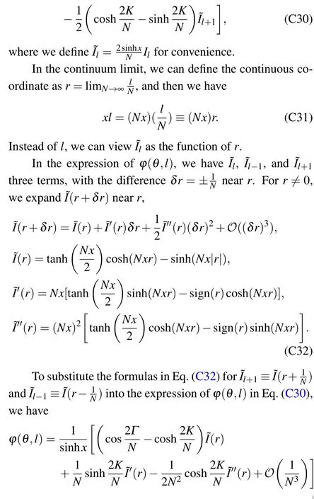
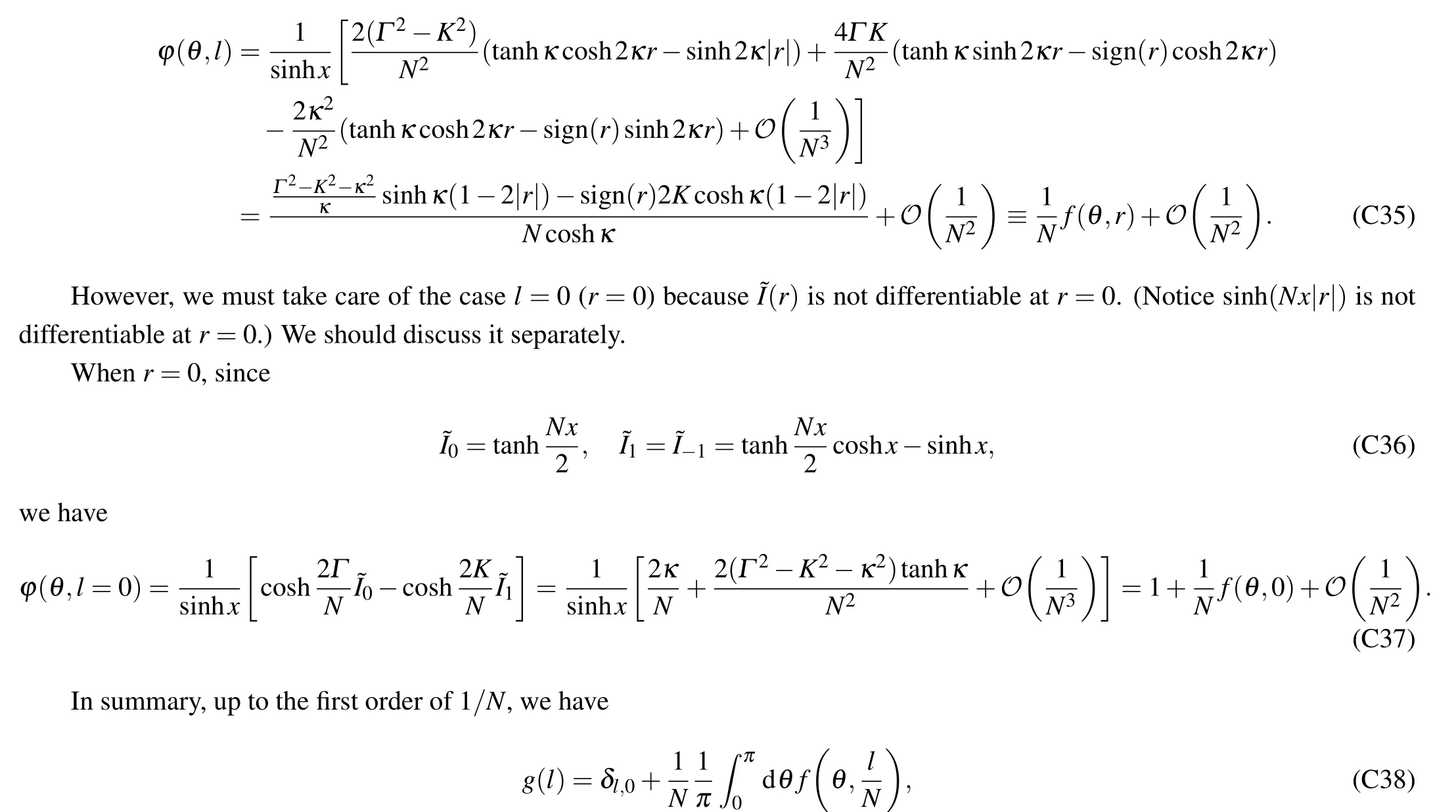
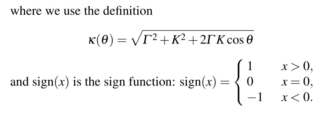
C5. Derive integral equation

With the preparation of the above subsections,we can finally derive the integral equation of the correlation matrix in the continuum limit. We consider the subsystem with ratioΛ=β′/β ∈[0,1]. The continuum limit can be realized as follows. We assume under certain trotter stepτ,the total system hasNfermion modes and subsystemMfermion modes,which satisfies

As the result, the eigen-equation of the correlation matrix becomes an integral equation in the continuum limit. The corresponding entanglement entropy is given by Eq. (36), as described in the main text.

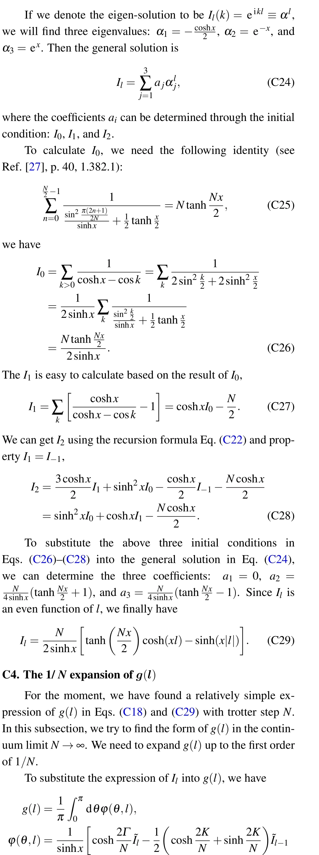
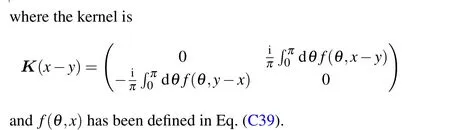
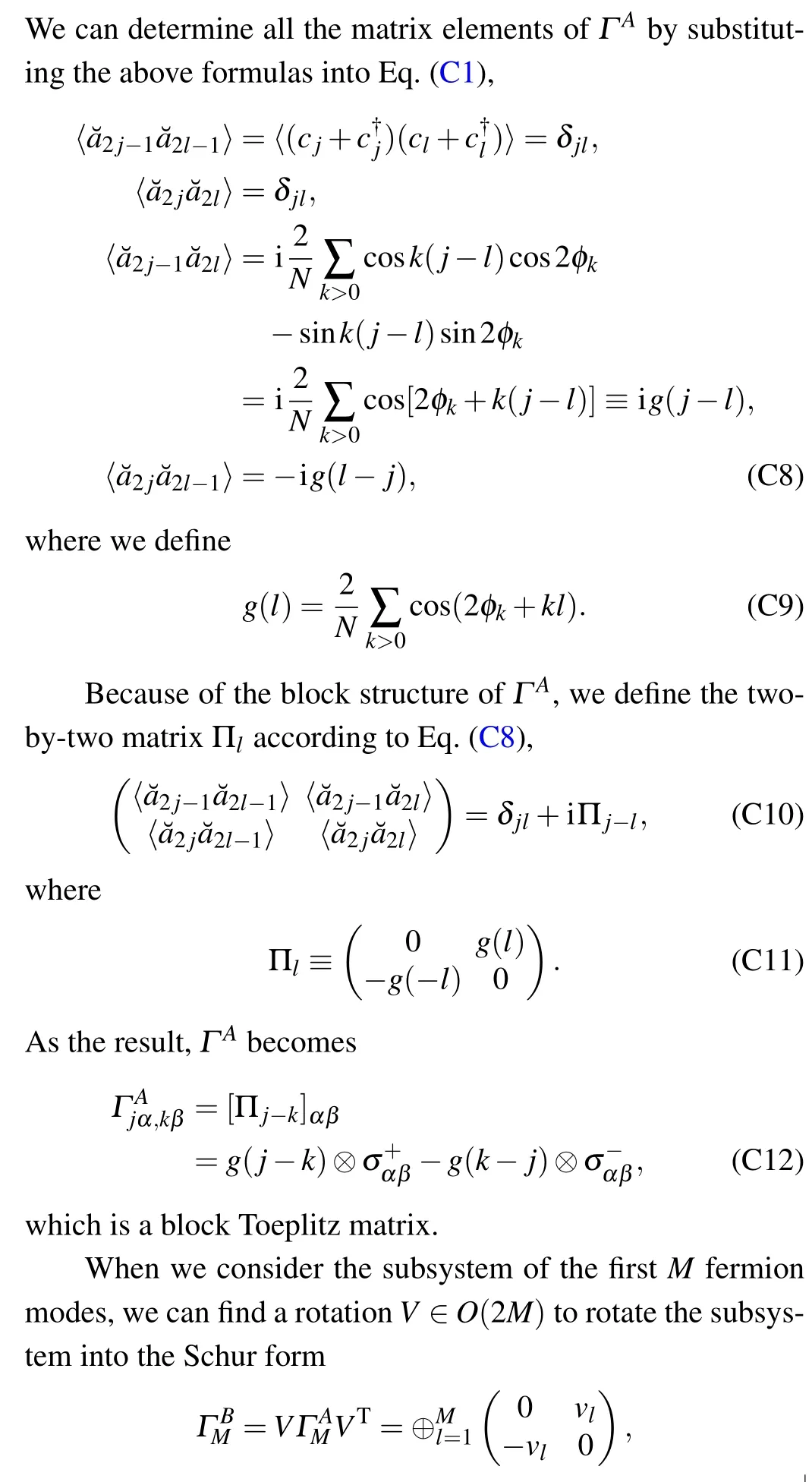
Appendix D:Ground state correlation at the continuum limit

The ground state of TFIM’s cMPO is a fermion Gaussian state, which is completely captured by its two-point correlation functions:〈ψ(x)ψ(y)〉,〈ψ?(x)ψ(y)〉,〈ψ?(x)ψ?(y)〉and〈ψ(x)ψ?(y)〉.

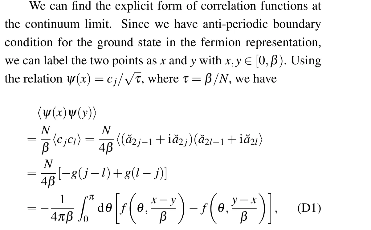
where, in the second equality, we use the transform relation Eq. (C1) between the fermion and Majorana representation;while in the last equality,we use the 1/Nexpansion ofg(l)in Eq.(C38).

To substitute the definition off(θ,x)into the above equation,we finally have

We can calculate〈ψ?(x)ψ?(y)〉and〈ψ(x)ψ?(y)〉following the same routine. However, using the commutation relations, we can easily find〈ψ?(x)ψ?(y)〉=-〈ψ(x)ψ(y)〉and〈ψ(x)ψ?(y)〉=δ(x-y)-〈ψ?(x)ψ(y)〉.

Appendix E:Exact cMPS representation ath=0

E1. Exact cMPS

Ath=0,TFIM reduces to the classical 1D Ising model

Acknowledgements

Y S. Z would like to thank Wei Tang for making me aware of the inspiring paper[8]and enlightening conversations. This project is supported by the Strategic Priority Research Program of the Chinese Academy of Sciences (Grant No. XDB30000000) and the National Natural Science Foundation of China(Grant Nos.11774398 and T2121001).