Quantum properties near the instability boundary in optomechanical system

Han-Hao Fang(方晗昊) Zhi-Jiao Deng(鄧志姣) Zhigang Zhu(朱志剛) and Yan-Li Zhou(周艷麗)

1Department of Physics,College of Liberal Arts and Sciences,National University of Defense Technology,Changsha 410073,China

2Interdisciplinary Center for Quantum Information,National University of Defense Technology,Changsha 410073,China

3Department of Physics,Lanzhou University of Technology,Lanzhou 730050,China

Keywords: optomechanical system,instability boundary,transitional region,quantum properties

1. Introduction

Optomechanical system,[1]which concerns the mutual interaction between radiation field and mechanical vibration,has received a lot of research interests. As the ground state cooling technology of the vibrator matures,[2,3]the study of the system’s quantum properties at low temperatures becomes particularly important. One of the interesting parameter regions lies near the instability boundary, where the mechanical vibration evolves into self-sustained oscillation once crossing the boundary into unstable region.[1]Studies show that driving the system near the instability boundary would enhance the nonlinearity at single-photon level,[4]increase the quantum entanglement,[5]or exhibit divergent susceptibilities,which is good for quantum sensing.[6]Therefore, it is worthy to make clear its general quantum properties near the instability boundary.

In a previous work,[7]the common features, in particular the changing of quantum entanglement,while crossing the instability line by different parameter paths have been studied.Under the current situations of weak optomechanical coupling and strong laser driving in experiments,[8]the mean-field approximation[1]has to be adopted due to the huge intractable Hilbert space involved in solving master equation. The main idea is to assume small quantum fluctuations around the classical orbit represented by the mean values of quantum operators,and then do the standard linearization.[9,10]However,the results obtained have two limitations.One is that there is a tiny region close to the boundary where the fluctuations diverge,[7]and the other is that it ignores the system’s non-Gaussian nature and can not show the characteristics of phase diffusion.[11]

The numerical solution of master equation can be possible in the single-photon strong coupling and weak driving regime,[12-16]where the optomechanical coupling strength is comparable to both the cavity decay rate and the mechanical frequency. Strong nonlinear effects such as photon blockade,[12]multiple sidebands in cavity output spectrum,[13]statistical mixture of two different oscillation amplitudes,[13,14]negative mechanical Wigner distribution,[15,16]sub-Poissonian mechanical states,[17]and Fano factor peak at phonon number threshold[18]have been discussed. But how are these nonlinear effects in parameter space related to the instability boundary, far away or nearby?Whether there are common features beyond the mean-field approximation when crossing the instability boundary?

The main purpose of this paper is to find out the general quantum properties near the instability boundary by numerical simulation of master equation. To do that,the system parameters should be adjusted to the regime of strong coupling and weak driving. Meanwhile, the classical orbits of mean values are depicted for comparison. The calculations show that while crossing the instability boundary from the stable region,the reduced mechanical state develops from Gaussian state to ring state with non-Gaussian transitional state connecting them. The Wigner distribution of transitional state directly reflects its bifurcation[19]behaviors in classical dynamics.There are typically two types: the supercritical Hopf bifurcation,and the saddle-node bifurcation followed by a subcritical Hopf bifurcation.[19]The transitional parameter region usually centers around the instability boundary, however, it might shift completely into the stable region where the saddle-node bifurcation takes place. In contrast to our initial intuitive,the transitional region instead of the vicinity of instability boundary is more fundamental. Its parameter width,position and bifurcation type can all be indicated by the mechanical second-order coherence function[20]and the optomechanical entanglement,and most importantly,the steady-state quantum entanglement in this region is very robust to thermal phonon noise. These results have revealed the general quantum features of optomechanical system near the instability boundary,many of which are missing in the mean-field approximation, thus also give some hints to rethink about the previous results[7]in the weak coupling regime.

The paper is organized as follows: In Section 2, after a brief review of the two-mode optomechanical system, the steady-state distribution on a two-dimensional stability diagram is presented. In Section 3, the transitional parameter region is focused for analysis, including its width and relative position to the instability boundary, two different types of bifurcations and their connection with mechanical Wigner distribution. The cross-boundary behaviors of the mechanical second-order coherence function and the optomechanical entanglement are discussed concretely in Section 4. Finally,the summary is given in Section 5.

2. Model and state distribution

The two-mode optomechanical system, which contains only one optical mode and one mechanical mode, has been studied thoroughly in many aspects.[1]Its Hamiltonian takes the following form in the rotating frame of driving laser frequencyωL:[21]

with mean valuesa ≡〈?a〉,qc≡〈?q〉,pc≡〈?p〉, andγm,κdenoting the mechanical damping rate and the cavity intensity decay rate respectively. The nonlinear dynamics of Eq.(2)has been widely studied including bistability,[23]limit cycles,[24]chaos,[25]etc. By letting all the first-order derivatives be zeros,the fixed points of this equation can be solved. The fixed point is stable (unstable) if it can attract (repel) any arbitrary close trajectories in phase space.[26]When driving the system with blue laser detuning (Δ ＞0) and large enough driving amplitude, the fixed point loses its stability to produce selfsustained mechanical oscillations,[14]and the vibrator undergoes periodic oscillation in the formqc=q0+Acos(ωmt)with shifted equilibrium positionq0and amplitudeA. The instability boundary has been found by demanding that the total mechanical damping rateγeff=γm+γopt=0,withγoptbeing the optomechanical part induced by radiation pressure.[1]γoptcan be positive or negative, which can either increase or decrease the total mechanical damping rate. In the blue-detuned regime,γoptis negative, decreasing the total damping rate. ifγeff=γm+γopt＜0,it can lead to amplification of thermal fluctuations and the system becomes unstable. So the boundary line approximately satisfies

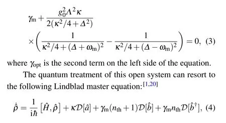
where ?ρis the density operator of the optomechanical system,D[?o]= ?o?ρ?o?-(?o??o?ρ+?ρ?o??o)/2 is the standard Lindblad operator,andnth=[exp(ˉhωm/(kBT))-1]-1is the mean thermal phonon number at temperatureT. To make it in a solvable small truncated Hilbert space, the system parameters in Ref.[7]can be changed to reach the instability boundary with very low laser driving amplitude by such a way that,g0is increased andωmis decreased by an order of magnitude respectively, andγmis reduced by three orders of magnitude. The maximum dimension of truncated Hilbert space in Fock-state basis|l〉opt?|n〉mecis about 4×350 or 3×500,which is manageable with QuTiP[27]on a computer server. The number of truncated phonons is increased to 380 or 520 respectively to test the convergence and the calculations remain unchanged,indicating that the number of truncated phonons is sufficient.The distribution probability on|0〉optexceeds 99%, while the distribution probability on|1〉optor a higher state is on the order of 10-3or even smaller. Therefore, the number of truncated photons is also sufficient.

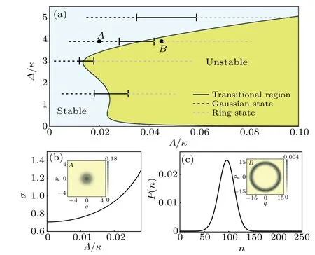
Fig.1. (a)Steady-state distribution on a two-dimensional stability diagram according to the mechanical Wigner distribution, where parameters used are g0/κ =0.5,ωm/κ =3,and γm/κ =10-5. The color division diagram of stability is the result of numerical calculation,while the black boundary curve is given by Eq. (3). Four horizontal paths that cross the boundary correspond to the drive detuning Δ/κ = 1.5,3, 3.9, 5 from bottom to top, respectively. Every path is divided into three regions: the solid black line represents the transitional region;the whole region on its left and right side is respectively Gaussian state(the dashed black line) and ring state (the dashed gray line). (b) Standard deviation σ of Gaussian states as a function of driving amplitude with Δ/κ =3.9. (c)Phonon number distribution for point B. The insets in panels(b)and(c)are the mechanical Wigner distributions for points A and B respectively, with their long-time classical orbits marked in red,the same marking for all the following Wigner functions.

3. Transitional region and bifurcations

This section mainly focuses on the change of the mechanical Wigner distribution function in the transitional region. To help understand these changes,the classical bifurcation behavior of the system is also given for comparison.

Fig. 2. (a) Changes in mechanical Wigner distribution in the transitional region with its corresponding bifurcation in the first type,where Δ/κ=3 and other parameters are the same as in Fig.1.The transitional region is marked by the shaded part.(b)Comparison of phonon number distribution for points C,D,E,and F.

In order to clarify the influence of parameters on width of the transitional region, the effect brought about by changing a certain parameter in Fig. 2 can be analyzed. The main results are demonstrated in Fig.3.When the non-sideband resonant drivingΔ/κ=1.5 is selected,the optomechanical interaction efficiency becomes weakened,the amplitudeArises relatively slowly, and the parameters that are farther away from the threshold point are required to form a ring state, so the width gets wider. When reducing the optomechanical coupling strength by 2.5 times tog0/κ=0.2, the thresholdΛthwill increase by 2.5 times, and the scale of amplitudeAwill also increase by 2.5 times,but the width of the noise will not increase by the same factor as the amplitude,which leads to a relatively smaller width of the transitional region.PointGcorresponds to pointFin Fig. 2. Its horizontal axis and vertical axis are both increased by 2.5 times,but it is in the ring state.If the mechanical damping rate is increased by 100 times to beγm/κ=10-3, the thresholdΛthwill increase by 10 times.These two factors cancel each other to maintain the vibrator’s amplitude scale and the noise width unchanged,so the relative width of the transitional region remains unchanged.Therefore,the key points to reduce the transitional width are to reduce the optomechanical coupling strength and select blue-sideband resonant driving.

In addition,when the amount of detuningΔ/κis greater than 3.8, the feature of blob-annulus coexistence Wigner distribution appears in the quantum state transitional region. This is related to another two consecutive bifurcation behaviors.[19]First, a saddle-node bifurcation occurs in the stable region,which is accompanied by a transition from a single stable fixed point to an additional pair of stable and unstable limit cycles of almost equal size. As the driving amplitude continues to increase, the size of the stable limit cycle increases, while the size of the unstable limit cycle decreases. Until reaching the instability boundary, the unstable limit cycle merges with the stable point and a subcritical Hopf bifurcation occurs,which makes the stable point unstable,while the previous stable limit cycle remains. Between the two bifurcations is the coexistence interval of a stable fixed point and a stable limit cycle. The quantum and classical correspondences of this coexistence phenomenon are fuzzy when the amount of detuning is small. As an example in Fig.4(a)withΔ/κ=3.9, pointIis a coexistence parameter point in the classic description,but its mechanical Wigner distribution looks like a blob. PointsJandKhave only one stable limit cycle, but theirP(n) distributions have two extreme values,and there will be an obvious blob-annulus coexistence Wigner distribution between them.

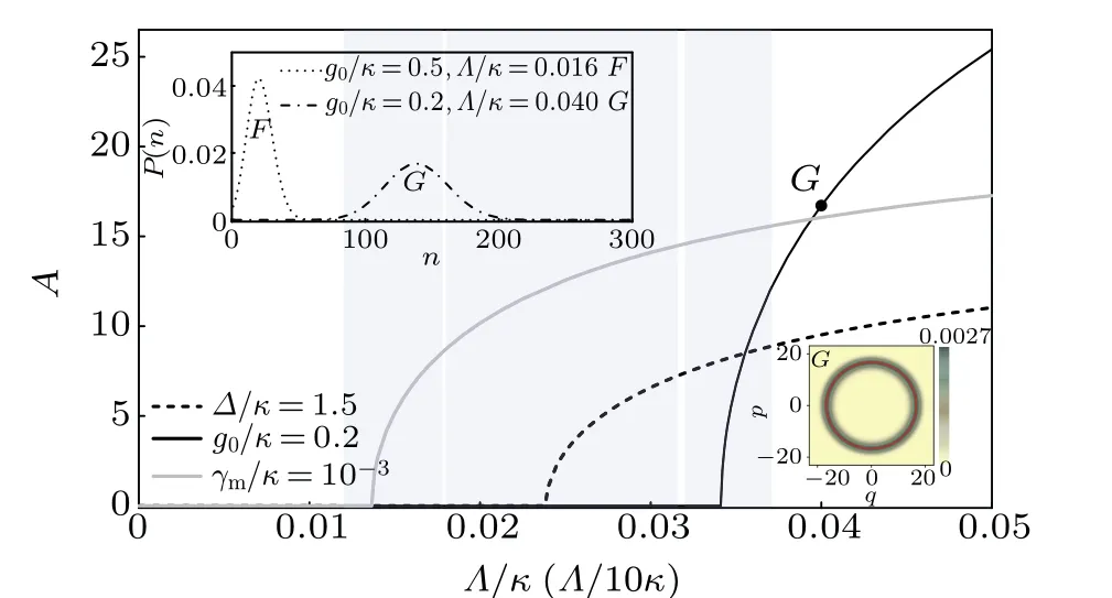
Fig.3. Influence of parameters on width of the transitional region,with the same parameters as in Fig. 2 excepted the one marked in the plot.The bifurcation curve for γm/κ =10-3 is rescaled 10 times smaller in the horizontal axis. The insets include the comparison of phonon number distribution for points F and G, and the mechanical Wigner distributions for point G.

Fig.4. Changes in mechanical Wigner distribution in the transitional region with its corresponding bifurcation in the second type,where Δ/κ =3.9 in(a)and Δ/κ =5 in(b)and other parameters are the same as in Fig.1. The color of the bifurcation curve represents the stability of the fixed point,light blue indicates stable,and red indicates unstable in order to mark the instability boundary. Each panel has insets to show the phonon number distribution and mechanical Wigner distribution for four selected points.

When the driving detuning is increased,the classical coexistence interval increases significantly,and the quantum and classical descriptions have a very good correspondence. In Fig.4(b)withΔ/κ=5,due to the relatively large size of the limit cycle in the first bifurcation,there are two completely independent peaks inP(n)that are far apart,and their statistical weights shift from one to another quickly within a small parameter range. So the coexistence phenomenon in the Wigner distribution only obviously occurs in a small range near theMpoint. In a large classical coexistence interval just before the instability boundary,the quantum states are completely in the ring states,such as theOpoint,whoseP(n)is a Gaussian distribution centered onn ?200.Due to the statistical weight,the transitional region completely breaks away from the instability boundary and enters the stable region.

4. Indications of transitional region

The transitional region serves as an important link between the Gaussian states and the ring states. For different bifurcation behaviors,in addition to the different changes in the Wigner distribution function,what other quantum features will it have? This section mainly discusses the cross-boundary behavior of two physical quantities,i.e.,the mechanical secondorder coherence function and the optomechanical entanglement.

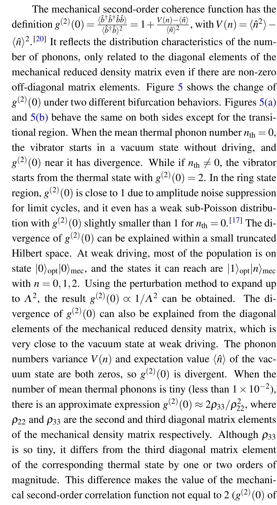
Fig. 5. Cross-boundary behavior of the mechanical second-order coherence function for two different bifurcation types,where Δ/κ =3 in(a)for the first type and Δ/κ =5 in(b)for the second type,and other parameters are the same as in Fig. 1. The overlapping shaded parts indicate multiple transitional regions. The larger the number of mean thermal phonons, the wider the transitional region. Red lines indicate the instability boundary.

In the transitional region, different bifurcations correspond to different changes ing(2)(0). For the first type of bifurcation,g(2)(0)decreases monotonically from a value close to 2 to close to 1. The parameter width of the transitional interval just corresponds tog(2)(0) in this value range. As the number of mean thermal phononnthincreases,the transitional interval widens,and the curve ofg(2)(0)becomes gentler(see Fig.5(a)). For the second type of bifurcation,due to the rapid transfer of statistical weight between the two peaks,the number of phonons increases sharply after the first saddle-node bifurcation as shown in Fig. 5(b). At the low end of the rising edge of the phonon number, there is a spike corresponding tog(2)(0), where the phonon number is small, but its variance increases significantly due to the two-peak structure,thus leading to a maximum. Along the rising edge,g(2)(0) drops rapidly because of the significant increase in the number of phonons. Whennthis increased,the weight of the small right peak in functionP(n) can be increased, so the rising edge of the number of phonons shifts to the left,while the peak value ofg(2)(0)shifts to the left and decreases. This is also accompanied by a widening of the transitional region and its center position shifting to the left.

Fig. 6. Cross-boundary behavior of optomechanical entanglement for two different bifurcation types,where Δ/κ =3 in(a)for the first type and Δ/κ =5 in (b) for the second type, and other parameters are the same as in Fig. 1. The extra gray curves in (a) give the results after γm/κ is increased by 100 times, their horizontal axis is reduced by 10 times, and vertical axis is reduced by 100 times for comparison. Another additional purple curve in(a)gives the result for decreasing g0/κ by 2.5 times, only its horizontal axis is reduced by 2.5 times for comparison.The oranges curves for nth=0 are obtained by the perturbation treatment in a small truncated Hilbert space,where photon numbers are{0, 1}, and phonon numbers are {0, 1, 2}, and expanding up to Λ2 terms. The overlapping shaded parts indicate multiple transitional regions with g0/κ=0.5,ωm/κ=3,and γm/κ=10-5 for different mean thermal phonon numbers. Red lines indicate the instability boundary with these parameters and the zoomed instability boundary with g0/κ or γm/κ changed.

When considering the influence of thermal phonon noise,the entanglement under weak driving decreases rapidly, and the entanglement in the ring state region also decreases significantly, but it still maintains a linear increase trend. The least affected is the transitional region, where the entanglement changes from a local minimum to a local maximum. As mentioned above,increasingγm/κby 100 times only enlarges the horizontal axis by 10 times, and the relative width and position of the transitional region remain unchanged. What’s more interesting is that the entanglement is only correspondingly increased by 100 times, and the changing curves with differentγm/κare very similar or even completely coincident(see Fig.6(a)). The entanglement curves corresponding to the second type of bifurcation are depicted in Fig.6(b). The outcomes are very similar, except that the entanglement in the transitional region has more subtle phenomena such as two bends and steps, anyhow, the entanglement in this region is also very robust to thermal phonon noise. For the weak coupling case, this entanglement robustness has also been found around the instability boundary.[7]It can be inferred that as the strength of optomechanical coupling increases, attention should be paid to the transitional region, which might be different from the region centered on the boundary line.

5. Conclusion

To summarize, the general quantum properties in a twomode optomechanical system near the instability boundary have been investigated by numerical simulations. According to the mechanical Wigner distribution, Gaussian states starting from the stable region will gradually evolve to the ring states deep in the unstable region after passing through a transitional region. The change of the mechanical Wigner distribution in the transitional region directly reflects its bifurcation behavior in classical dynamics. Besides, the cross-boundary behaviors of quantum properties such as mechanical secondorder coherence function, and optomechanical entanglement,are all closely related to the corresponding classical bifurcations. In turn, these quantum properties can be used to judge the corresponding bifurcation types and estimate the parameter width and position of the transitional region. For example,if a spike suddenly appears in theg(2)(0)function,it signifies that the saddle-node bifurcation in the second type of bifurcation has occurred, and the transitional region is an interval centered on this spike. The statistical weight also plays an import role,which might make the transitional region differ from the region centered on the boundary line. The former is more essential than the latter and its entanglement is very robust to thermal phonon noise,which are out of our previous expectation. In future applications, the transitional region should replace the instability boundary as the starting point for analysis and research.

Acknowledgements

Z. J. Deng is grateful to Liang Huang, Qiong-Yi He,Jie-Qiao Liao and Xiao-Bo Yan for useful discussions. This work is supported by the National Natural Science Foundation of China (Grant Nos. 11574398, 12174448, 12174447,11904402,12074433,11871472,and 12004430).