Scalar one-loop four-point integral with one massless vertex in loop regularization

Jin Zhang

School of Physics and Electronic Engineering, Yuxi Normal University, Yuxi, Yunnan, 653100, China

Abstract The scalar one-loop four-point function with one massless vertex is evaluated analytically by employing the loop regularization method.According to the method, a characteristic scale μs is introduced to regularize the divergent integrals.The infrared divergent parts,which take the form of and as μs →0 where λ is a constant and expressed in terms of masses and Mandelstam variables, and the infrared stable parts are well separated.The result is shown explicitly via 44 dilogarithms in the kinematic sector in which our evaluation is valid.

Keywords: one-loop four-point integral, loop regularization, dilogarithm

1.Introduction

The precise tests of physics within the framework of the Standard Model (SM) of particle physics and finding new physics beyond the SM always need to evaluate amplitudes of some physical process at quark level to higher orders of some coupling constant via perturbation theory.Analytic results of Feynman diagrams play a key role in investigating the infrared and ultraviolet structure of a theory but also in the ensuing numerical calculation.Methods of approaching this goal involve multi-loop or/and multi-point Feynman diagram evaluation.Up to now the particle physics community has developed powerful methods for higher-order Feynman diagram calculation, state-of-the-art techniques including integrating by parts [1, 2], evaluating by Mellin–Barnes representation [3], the differential equations method [4–10] and so on.For technical details of each approach and other rare methods,one can refer to[11–14]and the references therein.In evaluating Feynman diagrams we should realize that there is a significant difference in expressing the final results between massless and massive theories.In massless theories, the Feynman integrals can be expressed in terms of polylogarithms[15, 16].However, the evaluation of massive multiple-loop Feynman integrals are more complicated than the massless cases since the results cannot be expressed via polylogarithms,so the elliptic generalization of polylogarithms, so-called elliptic polylogarithms,are needed.Examples of this trend can be found in [17–25]; for the mathematical ground of elliptic polylogarithms and other properties, in particular the analytic structures, see [26–31].

The evaluation of one-loop integrals of Feynman diagrams holds a prominent position from both theoretical and experimental perspectives[32–35].It has been shown that the general N-point (N ≥5) scalar one-loop integrals can be recursively expressed in terms of combinations of (N ?1)-point integrals.Hence an arbitrary N-point (N ≥5) integral can be reduced to the sum of several scalar one-loop fourpoint integrals.Since tensor-type integrals can be reduced to scalar integrals by the Passarino–Veltman [36] scheme, we can obtain the desired results from scalar integrals by including appropriate tensor structures which are formed by metric tensor gμνand external momenta.Consequently, all types of one-loop integrals will be evaluated analytically in principle.In other words, scalar one-loop four-point integrals play an intermediate role that transits the intractable N-point(N ≥5) integrals to accessible ones.Therefore it is helpful to investigate the scalar four-point integrals carefully.

In the pioneering work by ’t Hooft and Veltman [37],scalar one-loop one-,two-,three-and four-point functions are studied generally and the scalar four-point function with real masses is expressed in terms of 24 dilogarithms, but for the case of complex masses it needs 108 dilogarithms.However,there is still a long way to go before the results can be used in practical applications.Subsequently, by using so-called projective transformation[37],it is found that the scalar one-loop four-point function can be reduced to 16 dilogarithms in some kinematical regions [38], and generalizations to tensor [39]and pentagon integrals [40, 41] are also carried out.An important application is made in [42] which employs box integrals to study some electroweak processes in the SM.A more complete work is given by[43]which calculates a set of scalar one-loop four-point integrals with massless internal lines and some massive external lines;the results obtained are convenient for analytic continuation.Scalar one-loop threeand four-point integrals for quantum chromodynamics are calculated in the space-like region in [44] where the ultraviolet, infrared and collinear divergent integrals are widely investigated.A thorough work in evaluating scalar four-point functions,which are valid for complex masses,is presented in[45], in which all the regular and soft and/or collinear singular integrals are analyzed by making use of dimensional and mass regularization.

Nearly all the scalar four-point integrals mentioned above are evaluated with the dimensional regularization method[46].An alternative way to extract singular parts in evaluating Feynman diagrams is loop regularization [47, 48], which has been successfully applied in some practical calculations in hadronic weak decays of B mesons [49–51].However, up toonly contributions of the so-called type-a and type-b diagrams to the amplitudes are considered in [49–51]; the evaluation of type-c diagrams is still lacking.If we want to include the contribution of type-c to the amplitudes,we must extract a scalar integral as depicted in figure 1.In other words,based on the integral corresponding to figure 1, it is possible to complete the evaluation ofcontributions to the amplitudes such that we may determine the branching ratios and direct charge–parity violation of B →ππ up tovia the six-quark operator effective weak Hamiltonian factorization approach,in order to be consistent with the evaluation of diagrams of type-a and type-b which are given in using loop regularization method.The advantage is that through the marriage of loop regularization and six-quark operator effective weak Hamiltonian factorization, it offers an alternative to evaluate the hadronic observables.

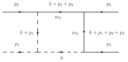
Figure 1.Scalar one-loop four-point integral with one massless vertex.The dashed and solid lines are massless and massive,respectively.As usual all the external momenta are inward.

On the other hand,noticing the significant role played by the scalar one-loop four-point integral in reducing the tedious N-point (N ≥5) integrals to tractable ones, it is helpful to study this diagram by loop regularization such that it provides some reference to the popular dimensional regularization scheme.The diagram under investigation in this paper,corresponding to‘Box 13’of[44],is collinear divergent1A analysis of soft and collinear divergence of a diagram with loop regularization via Cayley matrix will be presented in a separate publication..We know that the divergent structure of an amplitude is independent of the regularization scheme, but the expressions of the divergent part and the stable part may be distinct for different regularization schemes.Hence, we hope that by a specific example we may show how the infrared divergent and infrared stable parts are extracted via loop regularization.As far as we know there are many types of infrared divergent one-loop four-point integrals; however, in this paper we are not as ambitious as the aforementioned works on scalar oneloop four-point integrals which try to investigate the infrared integral of every type thoroughly, and instead we only focus on the diagram depicted in figure 1.In this sense we just present a case study on scalar one-loop four-point integrals by loop regularization.We hope that the results shed some light on the evaluation of scalar one-loop four-point integrals, but are also helpful in calculating some box diagram mediated decaying processes.

Before starting our evaluation, the following comments are in order.

(i) To perform the integrals over Feynman parameters, the Euler shift is adopted.Accordingly, two equations,i.e.,equations (32) and (61), should be satisfied by the transforming parameters α and β.We assume that the two equations have two real roots,and one root of each equation lies in the range (0, 1) as stated in our evaluation.These requirements fix a kinematic allowed sector in the space spanned by the masses and external momentum; we call it sector I.

(ii) In our evaluation we need to factorize 12 quadratic polynomials of F-type,which are denoted by Fij(i=0,1;j=1, 2, 3), and of G-type, which are denoted by Gij(i=0,1;j=1,2,3),into products of their roots.The Ftype functions are in the denominator and the G-type functions are arguments of logarithms; the coefficients of the two type functions are formed by on-shell masses and masses of propagators as well as invariant combination of external momentum.It is obvious that the factorization should be done carefully since it depends on if the quadratic polynomials have two real roots.In other words, the validity of each factorization determines a kinematic sector where the quadratic polynomial has two real roots.Hence,in all there are 12 kinematic sectors to be fixed, and the intersection of them is the kinematic sector where our evaluation is allowed, which we call sector II.Figuring out sector II exactly is difficult in the complicated space established by the masses and external momentum.In order to solve the dilemma, we assume that there may be some kinematic sector in which all the factorizations are valid.For a case-by-case analysis of similar integrals one can refer to the appendix of [52] and appendix D of [53].

The overlap of sector I and II is the desired kinematic part where the results obtained in this paper can be correctly applied.We assume that there is some method by which the overlapping sector can be determined, although we do not find it explicitly in this paper.It is worth emphasizing that the required kinematic sector may be unphysical or may not even exist;if this is the case,we just present a formal study on the infrared scalar one-loop four-point integral.

The paper is organized as follows.After this short introduction we display some mathematical functions which are frequently used in our evaluation in section 2.Then in section 3 details of the evaluation and results are presented.Section 4 contains our short summary.Some necessary formulae are listed in the appendix.

2.Preliminaries

We define the following massive scalar one-loop four-point integral with one massless vertex, as depicted in figure 1

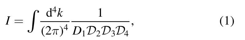
where

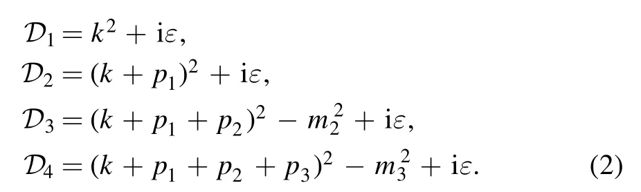
The iε will be systematically retained in our evaluation, and m2and m3are the masses of the two massive internal lines.As usual we fix all the external momenta as inward,and they are related by the energy conservation

We assume that the four external momenta satisfy

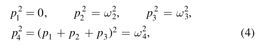
and for brevity we define

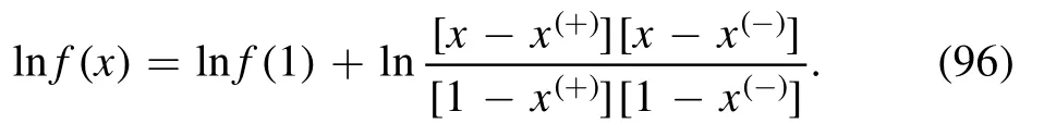
The results will be expressed in terms of logarithms and dilogarithms.As usual we choose for the principal value of the logarithms to lie in the negative axis; hence, we find

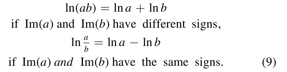
In expanding the logarithm of products one should take into account the convention [37]

where the η term is

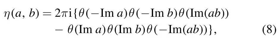
and following this rule it is easy to obtain

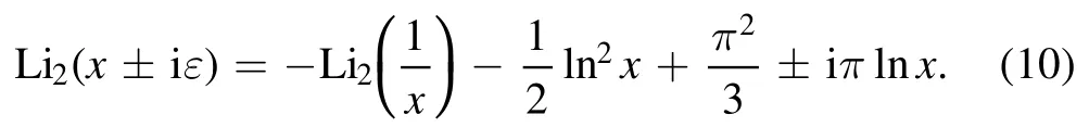
As we know the dilogarithm develops an imaginary part for x ≥1, we have [43]

Most of our results involve analytic continuation of dilogarithms of two variables

and this can be completed by the substitution [42, 45]

where η(x1, x2) is given by equation (8).

3.Calculation and results

3.1.Basic formula

First, we notice that the first two denominators can be combined via Feynman parameterization:

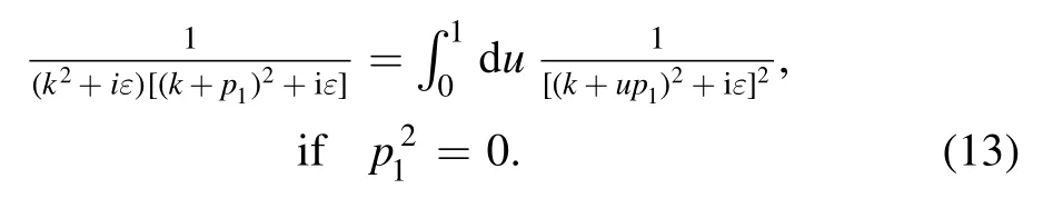
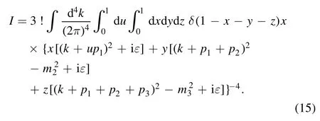
Then the primitive integral in equation (1) becomes

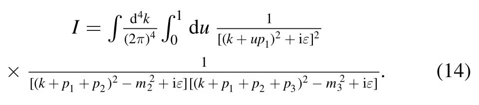
Then, by using Feynman parameterization twice,equation (14) can be written in the form

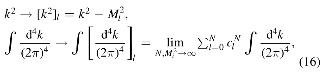
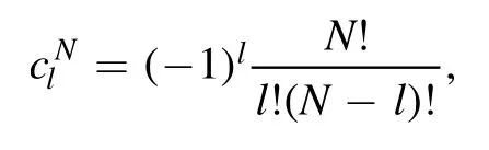
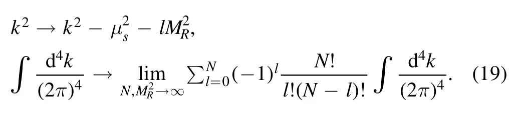
Sine there is infrared divergence in I,in order to carry out the integration over k,an appropriate regularization scheme must be employed.Instead of the most popular dimensional regularization, an alternative is loop regularization [47, 48].According to the method,the loop momentum k transforms as

which is constrained by

From equation (17) the coefficientscan be worked out:

and the regulator mass is given by

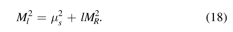
This then leads to the desired integration form over k:

If there is only infrared divergence,when the integration over loop momentum is completed,terms involving MRwill vanish after taking the limit;thus in this case it amounts to introduce a characteristic scale μsin the amplitudes.With this in mind,after the integration over k is performed, we obtain

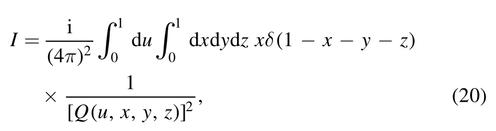
where Q is a polynomial defined as

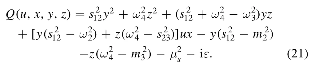
The integration over u is trivial and thus we do it first:

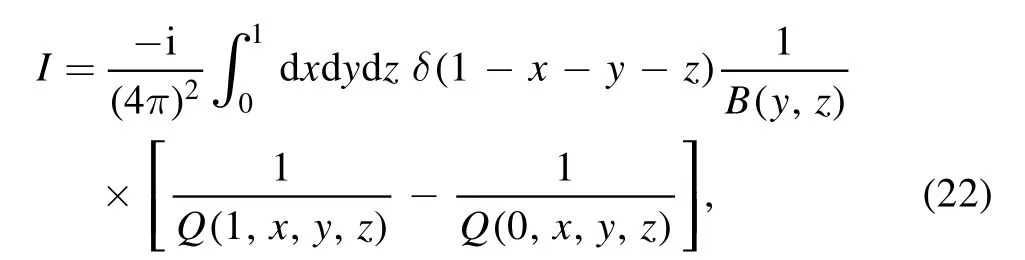
where

The integration over z can be performed immediately;it leads to

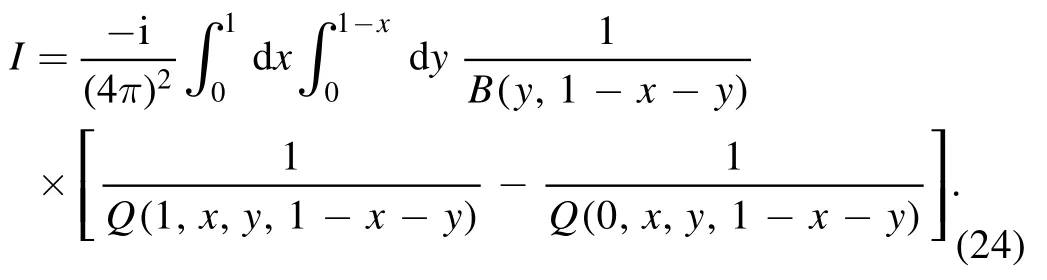
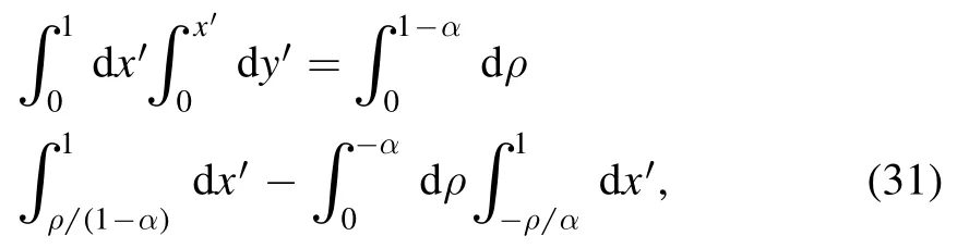
To proceed we make the following transformation on x and y:

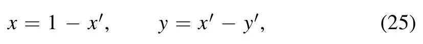
which yields a convenient form for equation (24):

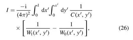
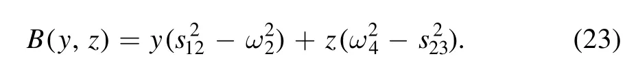
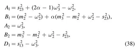
where

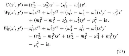
For later convenience we split I into two parts:

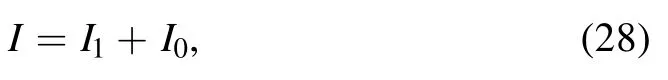
where the two components are

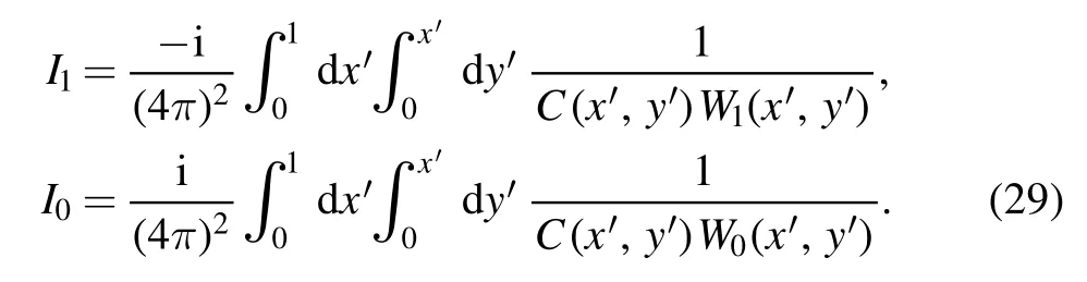
We will evaluate I1and I0in the forthcoming two subsections,respectively.

3.2.Evaluation of I1

Since the denominator W1is quadratic both inx′ andy′, in order to cope with terms involving x2, we perform the socalled Euler shift ony′:

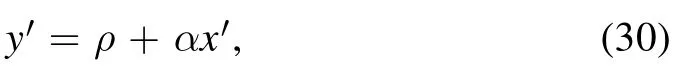
such that

where the parameter α is chosen to obey the condition

From equation (32) we find

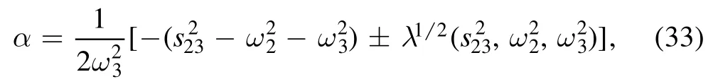
where λ(x, y, z) is the well-known K?llén function

In our evaluation we take

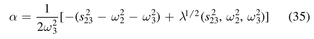
and assume 0 ＜α ＜1.According to equation (32), all thex′2Notice that the lower indices of f and g tell us the maximum power of ρ.-dependent terms vanish.Now that W1is linear inx′, we denote it as

where f1and f2only depend on ρ;the explicit expressions are2

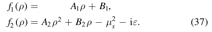
All the coefficients in equation (37) are constants which are formed by on-shell masses in equation (4) and propagator masses mi(i=2, 3) as well as combinations of external momentum sijin equation (5):

Under the transformation in equation (30), the functionC(x′ ,y′)becomes

where g0(α) is constant and g1(ρ) is linear in ρ:

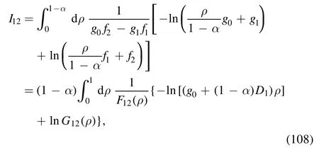
This yields a compact form for I1, which reads

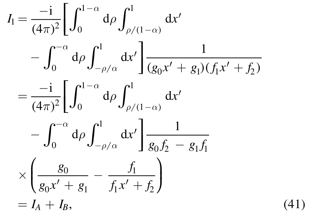
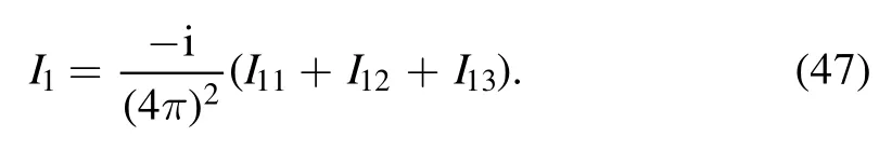
where we have split I1into two parts:

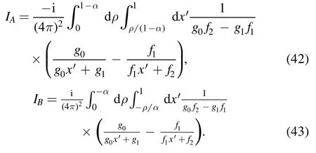
The integration overx′ in equations (42) and (43) is elementary and we can carry out it immediately;the results are

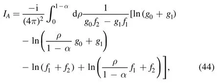
and

Then we divide the upper limit of the integral of IAinto two parts:

Combined with equation(45), after some cancellation we find

The first component I11is given by

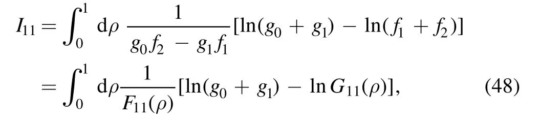
where

The other two components are

In order to regularize the upper limit of the integral in equation (50), we make the following variable substitution:

Without confusion,we relabel ξ as ρ;then the integral takes the form

where

Similarly, we make the following transformation in equation (51):

and relabel ξ as ρ, which leads to

where

The details of evaluating of I11, I12and I13are presented in appendix C.

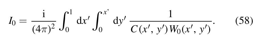
3.3.Evaluation of I0

The original expression of I0is

To eliminate the awkward term depending onx′2, we also make the Euler shift ony′:

such that

where β is chosen to obey the condition

which renders that all thex′2-dependent terms vanish.The roots of equation (61) are

where λ(x, y, z) is the K?llén function defined in equation (34).In our evaluation we take

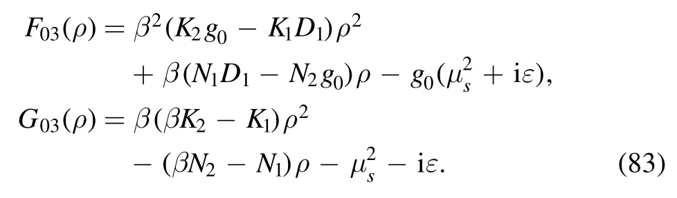
and assume 0 ＜β ＜1.Accordingly,W0is linear inx′ ,and we denote it as

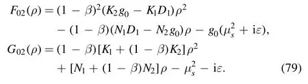
where the two functions h1(ρ) and h2(ρ) only depend on ρ;they are given by

where all the coefficients in equation (65) are constants:

whileC(x′ ,y′)transforms into

where g0(β) and g1(ρ) are given by

Then we rewrite I0in a compact form:

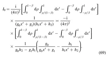
After the trivial integration overx′ is performed, we find

where

and

After some cancellation, we have

The first component is

where

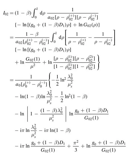
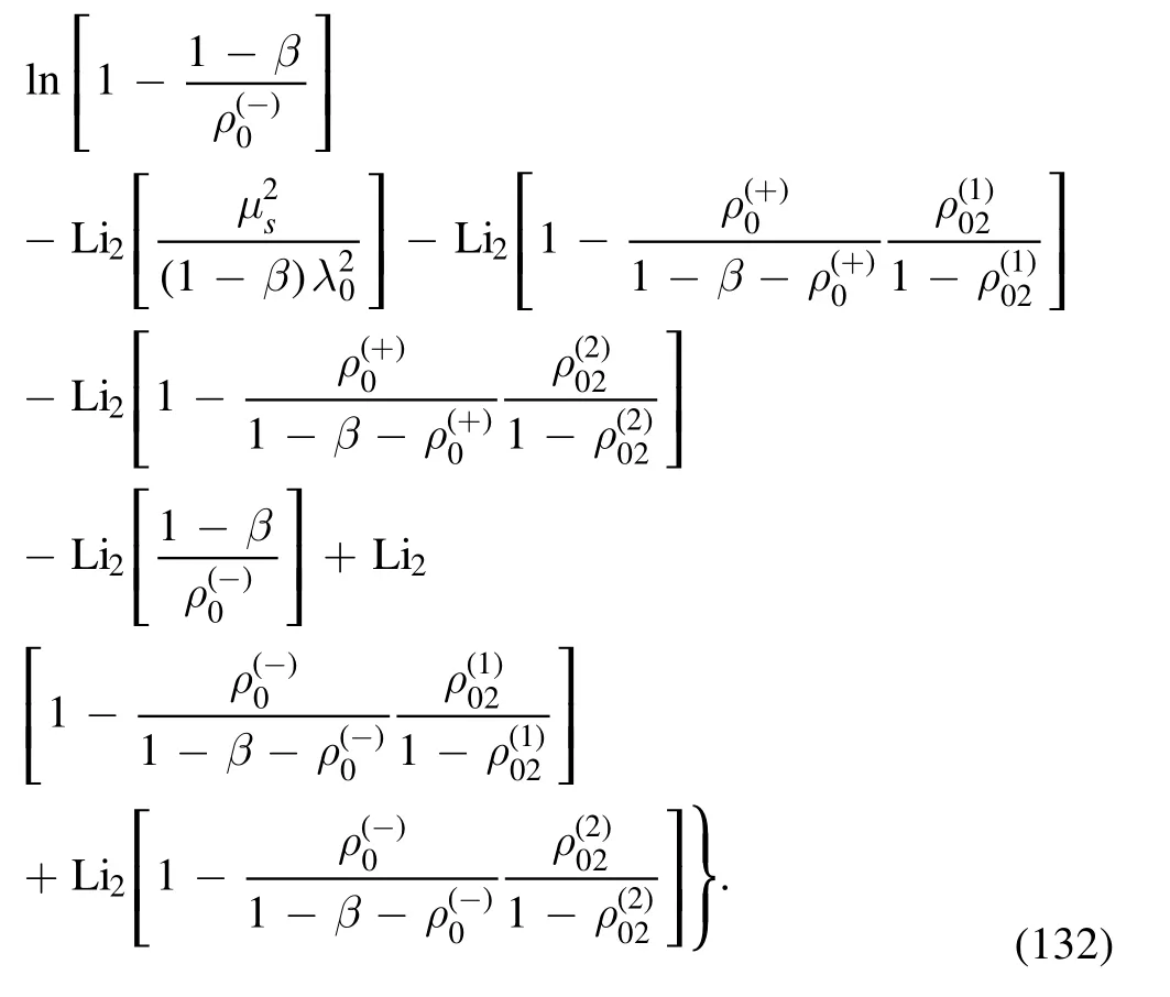
The second component is

We make the following transform on I02:

and relabeling ξ as ρ, we obtain

where

The last component is

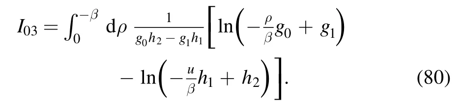
We make the following transformation:

and relabeling ξ as ρ,

where

The details of evaluating of I01, I02and I03are given in appendix D.

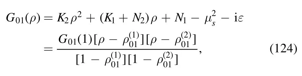
3.4.Results and discussion

Collecting the components in the appendices C and D, we arrive at the final results for I:

where the manifest expressions of I1and I1are

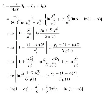
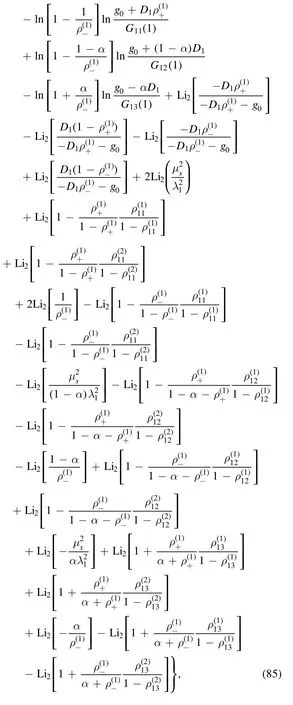
and

Combining equations(85)and(86),we obtain the final result for the integral in equation (1) in loop regularization.It is obvious that the infrared divergence appears as terms proportional toorwhen the characteristic scale μs→0.There are also infrared divergent and finite imaginary terms, which stem from analytic continuation of logarithms and dilogarithms by equations(6)and(10), respectively.As μs→0, the dilogarithms with arguments proportional toi.e.,in the form of Li2(where γ is a constant,will vanish.Since we hold the iε systematically in the evaluation, all the dilogarithms with two arguments of the form

can be expedient to make analytic continuation via equation (12).However, for brevity we retain the original form for every term like equation(87),otherwise there are too many terms to be listed.

It is meaningful to compare the results with some similar results obtained by the dimensional regularization scheme[44, 45].In the dimensional regularization scheme the final result in equation (1) may be expressed in a generic form as

where d is the dimension of space-time, coefficients A and B are complex functions of kinematic variables,and the terms in the infrared finite part are proportional to(n= 0, 1, 2,…).After the infrared cancellations,only terms independent ofare left in practical applications.In loop regularization, the infrared finite part depends on the characteristic scale μsbut μsis not fixed.This means that when μsis sliding,the infrared finite part is variable.Thus, when we analyze several processes based on loop regularization, if the result of each process is consistent with experiments for the same μs, it implies that the given μsis reasonable for these processes.

4.Conclusions

In this paper the scalar one-loop four-point function with a massless vertex is calculated analytically by loop regularization, and the infrared divergent and infrared stable parts are well separated.The results are convenient to analytically continue to other kinematic sectors which are beyond our assumption.Following the steps proposed in this paper, oneloop tensor-type four-point integrals are easy to evaluate.In particular, this will be beneficial for calculating complete contributions up to O(to the amplitudes via the six-quark operator effective weak Hamiltonian factorization approach.However,we should realize that since the kinematic region in which our results are valid is determined by 12 equations,as a result it greatly constrains the application of the final results.If the results obtained by an other regularization method(for instance, dimensional regularization), analytically or numerically, are valid in the same kinematic region as our paper, a cross check is feasible.A practical way of checking may be to apply the results to evaluate some specific decay processes, and then compare the evaluated results with the experiments.This will be one of our research works undertaken in the near future.

Acknowledgments

The author thanks H E Haber for helpful discussion on the properties of dilogarithms.

Appendix A.Factorization of quadratic equation with two real roots

Suppose f(x) is a quadratic polynomial with imaginary part

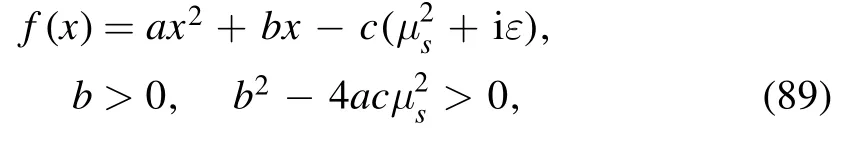
where ε is a real, positive infinitesimal.The two zeros of equation (89) are

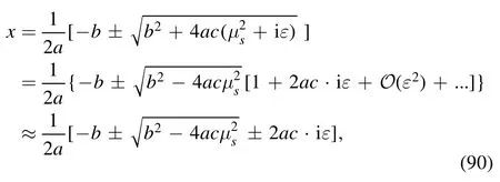
where we have used the property that the product of any finite quantity with ε is still a real infinitesimal,and we still denote it by ε.Supposing?1, we may expand the two zeros as power series of

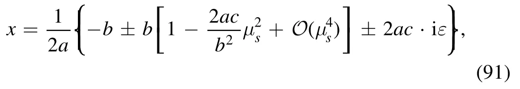
and then we get two roots:

Now we would like to factorize equation (89) as

and then we obtain

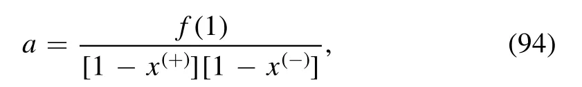
This leads to an useful factorization on f(x):

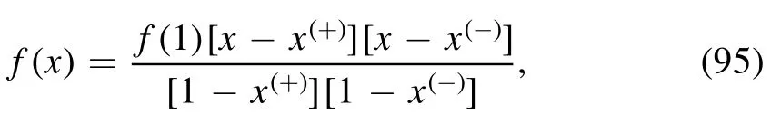
and assuming f(x) is real and f(1)＞0, according to equation (9), we find the useful expression below:

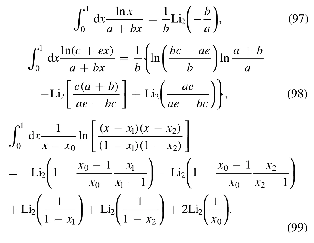
Appendix B.Useful auxiliary integrals

In this section we list some integral formulae which are useful in the calculation; they are taken from [44, 54].

Appendix C.Evaluating the three components of I1

In this section we present the details of evaluation of the three component of I1.In appendices C and D, equation (10) is frequently employed.In principle, dilogarithms with two arguments can be analytically continued by using equation(12),but for brevity we do not make the analytic continuation and just retain their original form.

· evaluation of I11

The integral is

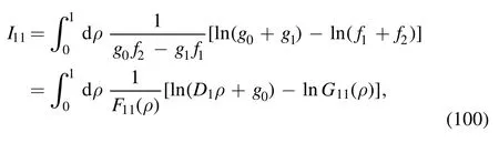
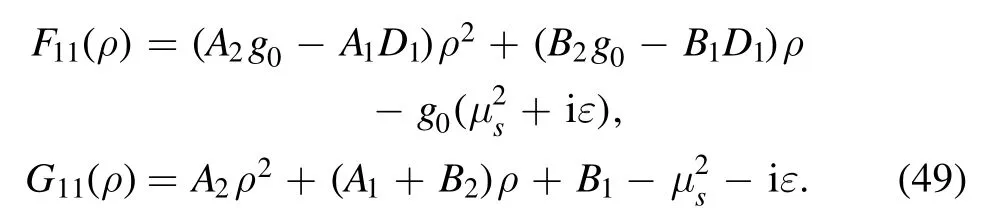
where the denominator F11(ρ) is quadratic in ρ:

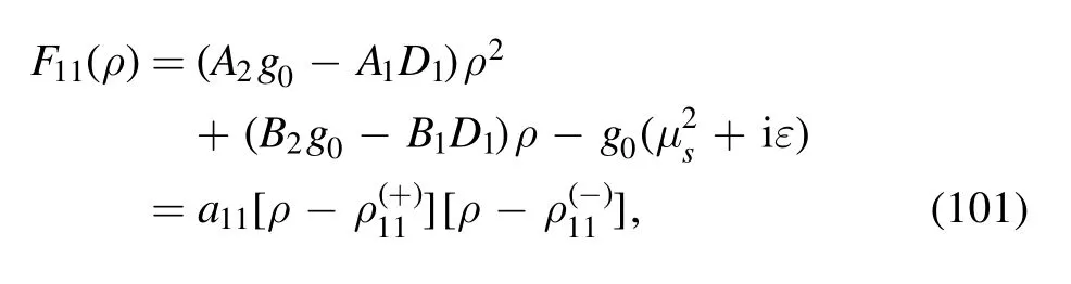
The two zeros in equation (101) are

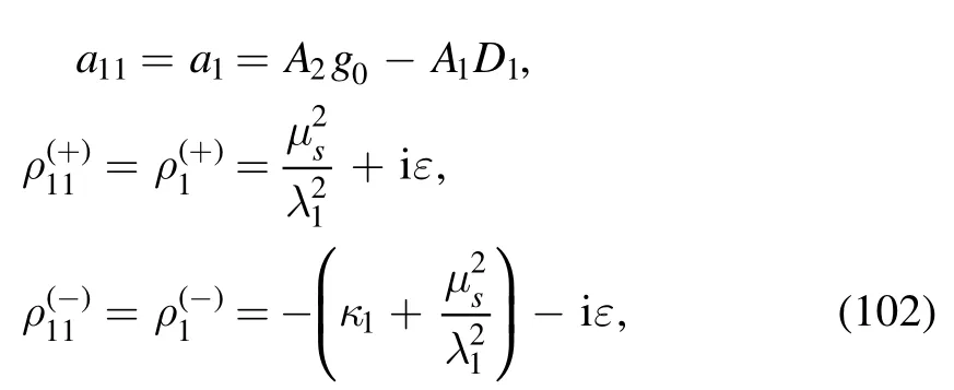
where in order to simplify the symbols,we have relabeled a11,respectively.The dimensional λ1anddimensionlessκ1aredefined as follows:

The manifest expression of G11is

By employing the equations in appendix A, it is not difficult to factorize G11into the product of its roots:

where

By using the formula in appendix B, we obtain

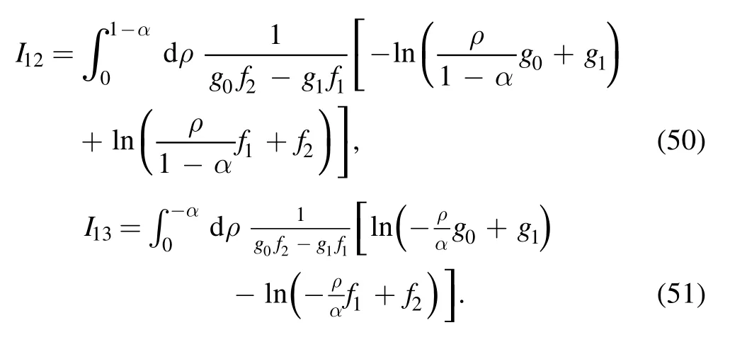
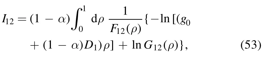
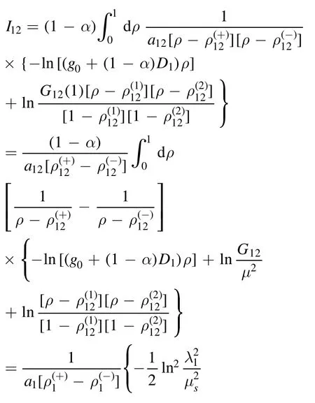
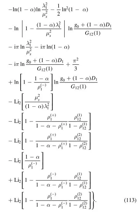
· evaluation of I12

After the variable substitution, the integral is

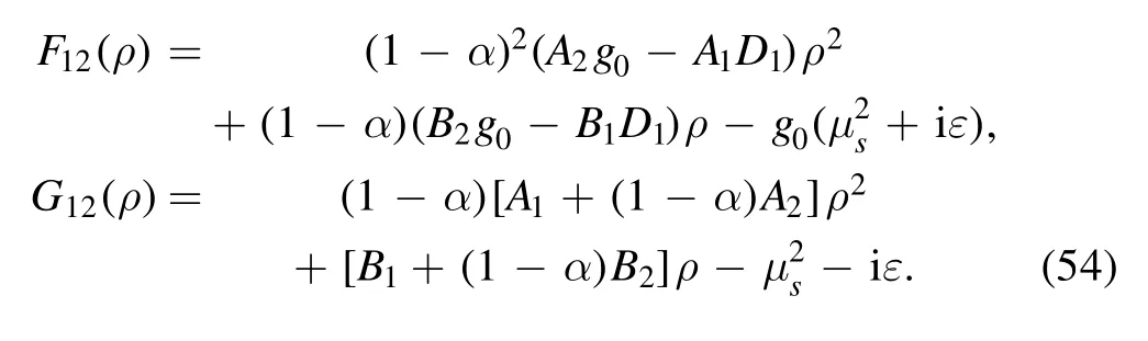
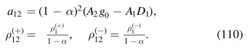
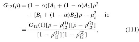
where F12(ρ) is given by

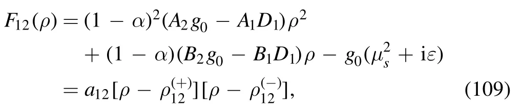
with

The argument of the second logarithm in the numerator is defined as

with

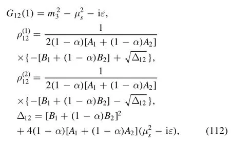
where equation (32) has been employed.By using the equation in appendix B, it is not difficult to obtain

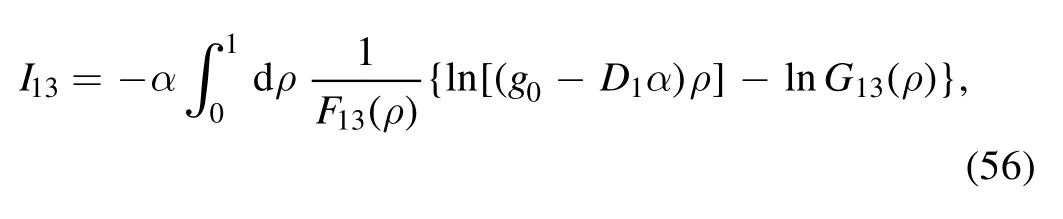
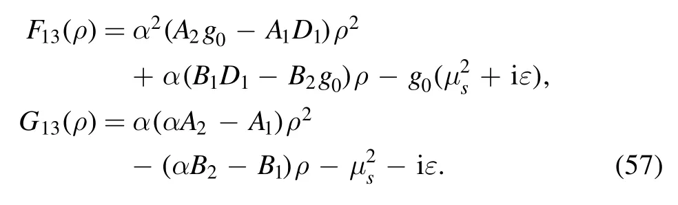
· evaluation of I13

The integral is

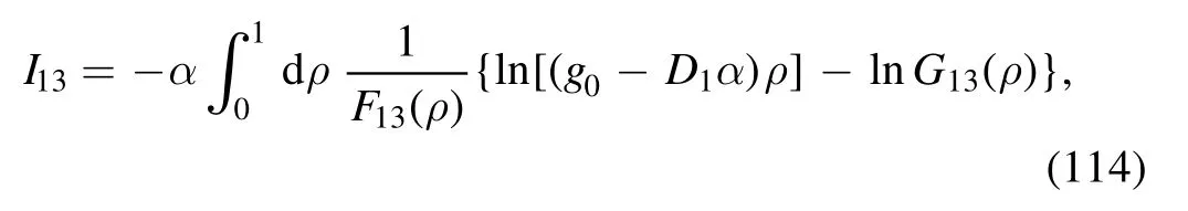
where

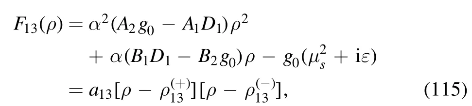
with

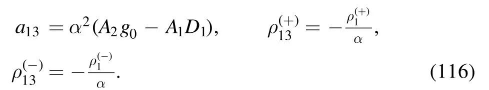
The argument of the second logarithm in the numerator is

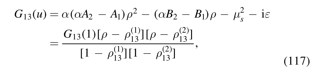
with

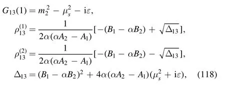
where equation (32) has been employed.By using the equations listed in appendix B, it is easy to obtain

Appendix D.Evaluating the three components of I0

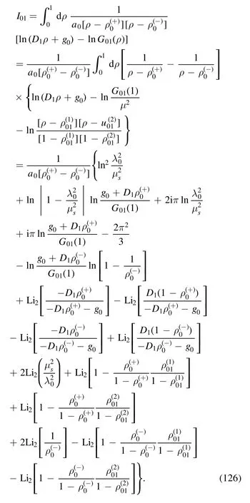
· evaluation of I01

The integral is

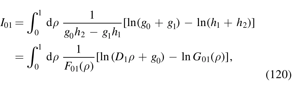
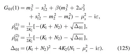
where the denominator is

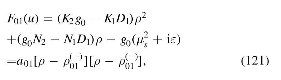
with

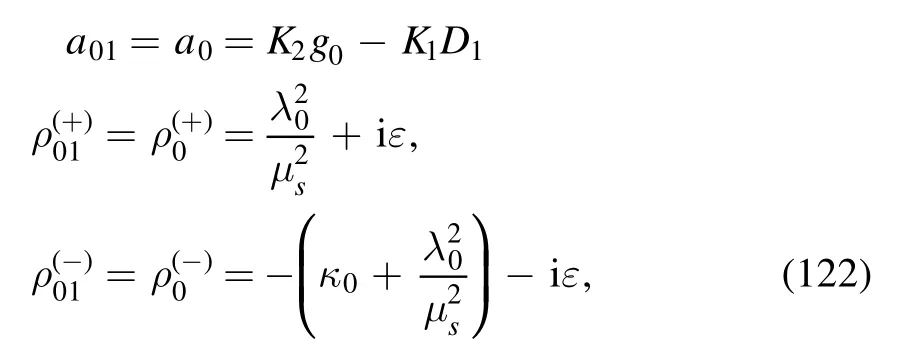
where in order to simplify the symbols,we have relabeled a01,andas a0,andrespectively.The dimensional λ0and dimensionless κ0are defined as follows:

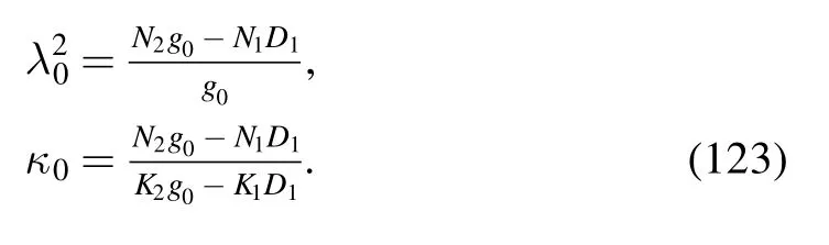
The argument of the second logarithm in the numerator is

with

With the help of the equations listed in appendix B, we find

· evaluation of I02

The integral is

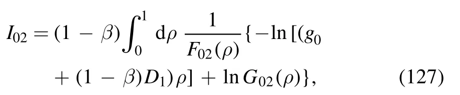
where the denominator is

with

The argument of the second logarithm in the numerator is

with

where equation (61) has been employed.By using the equations in appendix B,it is not difficult to obtain the result

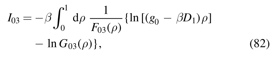
· evaluation of I03

The integral is

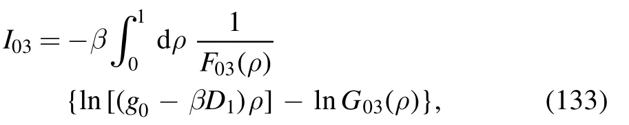
where we define

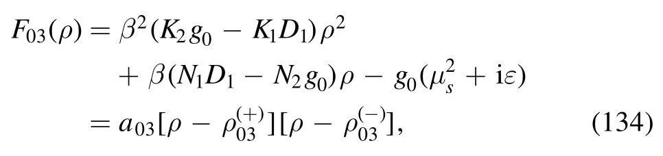
with

The argument of the second logarithm in the numerator is

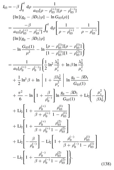
with

where equation (61) has been used.By employing the equations in appendix B we can obtain