Machine learning application to predict the electron temperature on the J-TEXT tokamak

Jiaolong DONG(董蛟龍),Jianchao LI(李建超),Yonghua DING (丁永華),?,Xiaoqing ZHANG (張曉卿), Nengchao WANG (王能超), Da LI (李達),Wei YAN (嚴(yán)偉), Chengshuo SHEN (沈呈碩), Ying HE (何瑩),Xiehang REN (任頡頏), Donghui XIA (夏冬輝) and the J-TEXT Team,3

1 International Joint Research Laboratory of Magnetic Confinement Fusion and Plasma Physics, State Key Laboratory of Advanced Electromagnetic Engineering and Technology,School of Electrical and Electronic Engineering, Huazhong University of Science and Technology, Wuhan 430074, People’s Republic of China

2 Hubei Key Laboratory of Optical Information and Pattern Recognition, Wuhan Institute of Technology,Wuhan 430205, People’s Republic of China

Abstract The reliability of diagnostic systems in tokamak plasma is of great significance for physics researches or fusion reactor.When some diagnostics fail to detect information about the plasma status,such as electron temperature,they can also be obtained by another method:fitted by other diagnostic signals through machine learning.The paper herein is based on a machine learning method to predict electron temperature, in case the diagnostic systems fail to detect plasma temperature.The fully-connected neural network, utilizing back propagation with two hidden layers, is utilized to estimate plasma electron temperature approximately on the J-TEXT.The input parameters consist of soft x-ray emission intensity, electron density, plasma current, loop voltage, and toroidal magnetic field, while the targets are signals of electron temperature from electron cyclotron emission and x-ray imaging crystal spectrometer.Therefore, the temperature profile is reconstructed by other diagnostic signals, and the average errors are within 5%.In addition, generalized regression neural network can also achieve this function to estimate the temperature profile with similar accuracy.Predicting electron temperature by neural network reveals that machine learning can be used as backup means for plasma information so as to enhance the reliability of diagnostics.

Keywords: neural network, plasma, electron temperature, J-TEXT tokamak

1.Introduction

Machine learning has been widely used in fusion research,such as plasma disruption prediction [1–3], fast magnetic equilibrium reconstruction [4], fast spectroscopic analysis [5],feature extraction [6], Non-power law scaling [7] and ideal stability properties prediction [8].In addition, it also has been used in plasma diagnostics for data processing[9],optimization[10] and temperature measurements.On W7-X, a neural network is utilized to approximate the full model Bayesian inference of plasma profiles from x-ray imaging diagnostic measurements [11].On the JET, plasma temperature can be predicted mainly by empirical transport models based on assumptions on the other profiles and plasma parameters [12]though they adopt neural networks to emulate the results of first-principle-based turbulent transport (QLKNN-4Dkin).

Besides the application of diagnostics and simulation,the neural network can fit the relation between different variables,namely, diagnostic signals on plasma information.For instance, soft x-ray emission intensityIsxrin plasma core is related with plasma parameters (effective ion chargeZeff, electron densityneand electron temperatureTe),indicating certain relation betweenTeand other signals likeIsxrandne.It can be expected that neural network could be able to make a fitting to estimate electron temperature by other signals, and then the fitting can predict electron temperature when no measurements ofTe.Based on above conjecture, different types of neural networks are utilized to reconstruct the relation betweenTeand other signals to predictTeon the J-TEXT tokamak [13, 14].On the J-TEXT, electron temperature is measured by the electron cyclotron emission (ECE) [15, 16] with high time resolution and by the tangential x-ray imaging crystal spectrometer(XICS)[17,18]with a time resolution of a few milliseconds.TheseTemeasurements might be unavailable occasionally.For example, XICS does not work routinely, and ECE is not operated for lacking protection from the electron cyclotron resonance heating(ECRH)system until shot#1065900 when the 105 GHz notching filter is well installed in the ECE system.In that case,the electron temperature predicted by neural networks may be beneficial to physics researches to some extent.

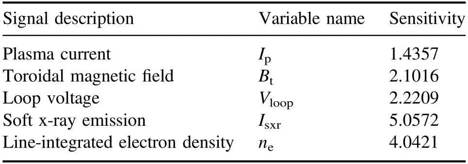
Table 1.Parameter list for input of neural networks.

In this paper, the machine learning methods and data preprocessing methods are introduced in section 2.Section 3 introduces the establishment of a single-channel temperature prediction model, and presents the results that two machine learning methods can predict electron temperature profile on ECE radiometer and XICS.Section 4 is the conclusion.

2.Algorithm model and data processing

In this paper, two types of neural network are employed for comparison, i.e.error back propagation neural network(BPNN) [19] and generalized regression neural network(GRNN) [20].They are based on the toolbox of machine learning in MATLAB 2017a.Training targets of both types are signals of electron temperature,Te, measured by the 24-channel ECE radiometer and XICS.Ruck sensitivity analysis method [21] is employed for analysis of the model parameters.This sensitivity coefficientsican reveal the degree of influence of input parametersxion output parametersy, i.e.If the sensitivity coefficient of certain parameter is small enough,this parameter has weak relation with the targetTe,and should be discarded from input parameters.Five input parameters and their sensitivity coefficients are listed in table 1.These 5 parameters are relevant toTe, and then selected as input parameters: plasma currentIp, toroidal magnetic fieldBt, soft x-ray emission intensityIsxr[22], lineintegrated electron densityne[23] from the polarimeter interferometer, and loop voltageVloop,as shown in table 1.It should be noted that when the input parameter Isxrcontains the values ofIsxr(tk) signal (r=0) at 9 time points

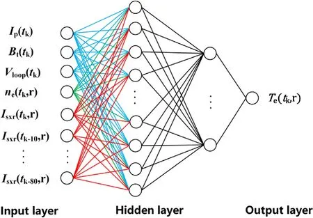
Figure 1.Schematic of the application of single-channel neural network.

The time interval between two adjacent points is 0.1 ms, and hence the size of the time window is 0.8 ms.The time window can better predict electron temperature and related physical phenomena probably because it likely relates to the time scale of instability.Isxr, including multipleIsxr(tk) signals at different times,contains equilibrium and perturbations caused by plasma activities and hence the electron temperature including perturbation caused by plasma activities like sawtooth oscillations can be accurately predicted;otherwise,with theIsxrat one time pointtkas input parameter, only the equilibrium temperature can be obtained while perturbations caused by plasma activities cannot be accurately predicted.

In order to demonstrate that BPNN and GRNN can be used to predictTemeasured by either ECE or XICS, two databases are established using the experimental data in J-TEXT campaign 2019 autumn: database A for the prediction of ECE signals employs data in shots #1066606?1066648, while database B for the prediction of XICS signals in shots #1064944?1065791.The sampling frequency of all signals is 100 kHz by down sampling and all samples are selected from signals during theIpflattop stage from 0.28 to 0.53 s.All the samples are normalized to the region of [0, 1].There are 1.7 million and 5.2 million data point samples in databases A and B respectively for predicting the ECE and XICS signals.It should be noted that the application shots of the network in section 3 are all excluded from the databases A and B.

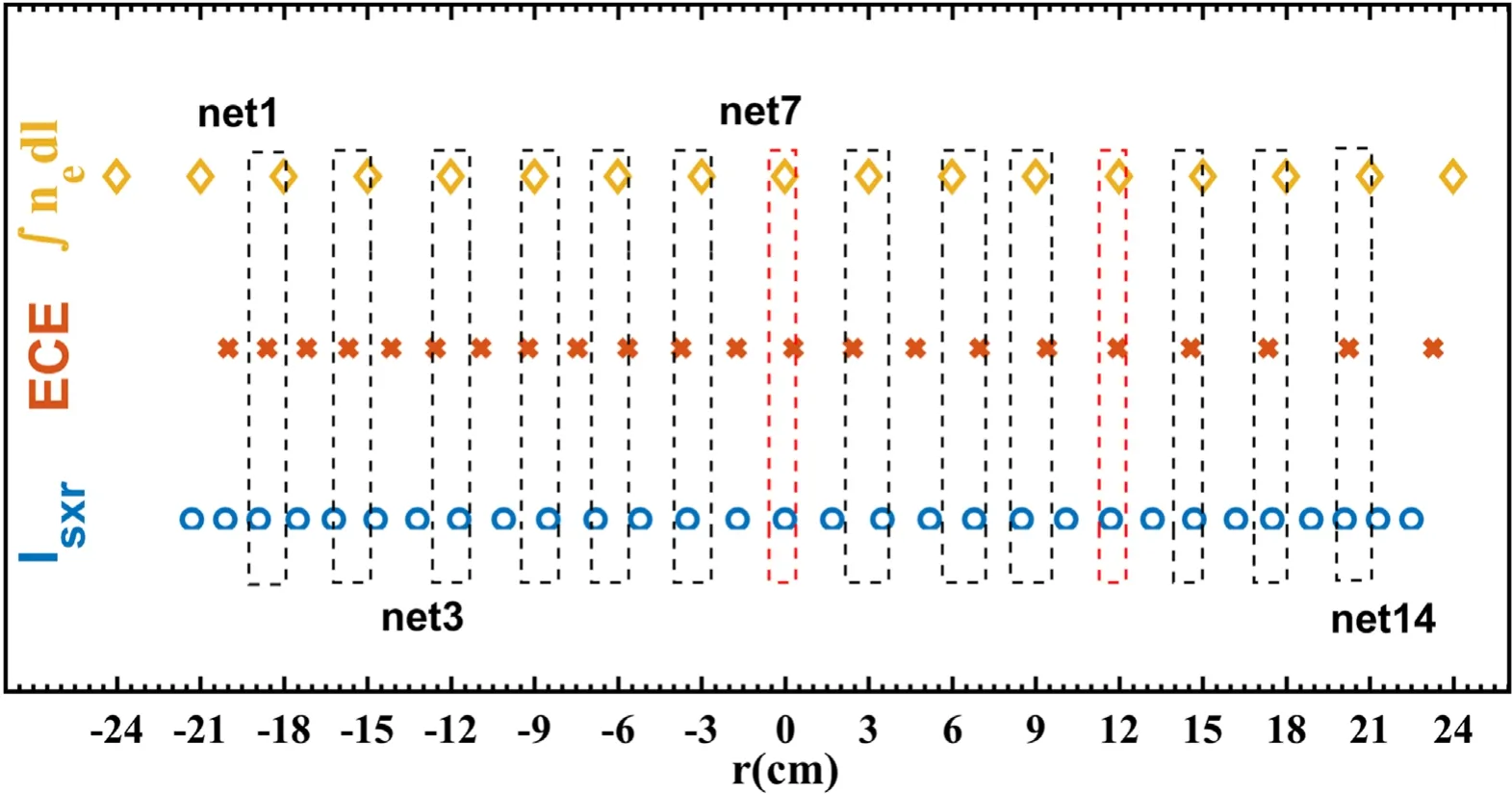
Figure 2.The detecting radii of ECE,SXR and polarimeter interferometer.The X axis is the position of the minor radius or chord radius of line-integrated signals.The radii of ECE are determined with Bt=1.8 T and marked by red crosses.Each dashed box marks one set of ne and Isxr as input parameters, and ECE signals as target.

In this work,BP neural network employs fully-connected neural network with two hidden layers,which have 15 and 10 neurons respectively,as shown in figure 1.We have tuned the parameters multiple times and it is found that these values can balance time and accuracy of training networks.The activation function isTan-Sigmoid,The target error is described by the mean square error(MSE).The MSE and mean absolute error (MAE) can depict the difference between fitting electron temperatureTeBPand normalized ECE signalsrevealing fitting accuracy of the network, and they can be determined by

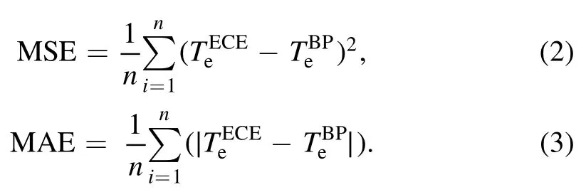
The process of training would end when the MSE value reaches the setting values(0.002 in this paper)or converges to the larger value.

The BP neural network is trained by functionfeedforwardnetin the toolbox of MATLAB.During training network,the Levenberg–Marquardt algorithm,as one method on solving extremum values of functions fast and accurately by iterative method, is employed in the functionfeedforwardnet.The algorithm combines fast convergence of gradient descent algorithm for slow descent and accurate convergence of Newton method for quick descent.In order to ensure the reliability and generalization performance of the model, the samples are divided into three parts: 70% of samplings for training, used to fit the parameters of the model; 15% for validation, used to tune the parameters; 15% for testing the generalization of the fully specified model.In this work,much effort has been made to avoid the occurrence of overfitting,like validation and testing of networks, reducing the numbers of neurons and the hidden layers,adjusting target error and so on.

The GRNN in this paper consists of two hidden layers,the radial base layer and summation layer.The radial base layer employs Gaussian function as kernel function for strong local fitting ability.The number of neurons in the hidden layer is equal to that of training samples,while the summation layer contains two neurons to calculate the algebraic sum and weighted sum of the output of the hidden layer neurons.The GRNN, trained by thenewgrnnfunction in MATLAB, has only one hyperparameter:Spread, which represents the spreading speed of the radial basis function.The smaller theSpreadvalue is, the more accurate the training sample point is.However, if the value is too small, overfitting will occur,thereby reducing the ability of model promotion.It is 0.004 for satisfying fitting in this paper.

3.Electron temperature prediction

On the J-TEXT, soft x-ray array system and polarimeter interferometer can provide the profiles of line-integratedIsxrandne, and their impact radii are shown by the blue circles and yellow diamonds respectively in figure 2.To preferably predict localTeat certain point, it is better to employ plasma information nearly this radial location to reconstruct their relation by neural networks.Therefore, 14 neural networks for predicting different positions were built.For instance,one neural network(net7 in figure 2)can reconstructTein plasma core byneandIsxrin plasma, while analogouslyTeat any other point can be reconstructed byne,Isxrand other parameters near this point.This section presents the training and application of neural networks (net7 and net12) in plasma core, and the prediction ofTeprofile by 14 neural networks marked by rectangular boxes in figure 2.

In database A, two typical shots with different MHD activities (sawtooth oscillations and tearing mode in shots#1066607 and 1066633, respectively) are selected for application of the networks, while the others are divided into training, validation and test samples to train the neural network to predict the ECE signals.The hyperparameters have been described in section 2.

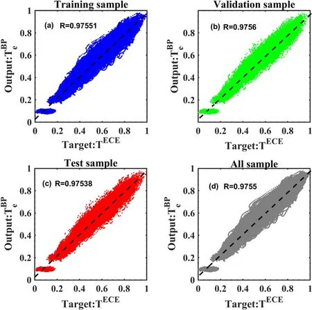
Figure 3.Predicted relative electron temperature corresponding to normalized ECE signals in (a) training sample, (b) validation sample, (c) test sample and in (d) all sample. R is the correlation coefficient.

When training net7 to predict ECE signals atr～ 0,after 222 epochs the MSE reaches the least value of 0.0023, andTeBPis highly linear toTeECEwith correlation coefficient of above 0.975 in train sample, validation sample, test sample and in all sample, simultaneously, as shown in figure 3.The MSE in the process of training is shown in figure 4.In this figure, the MSE values of validation (the green line) and test(the red dotted line) samples are similar to those of training(the blue circle) sample in all epochs.The model works well on training sample, and it also works well on test sample,reflecting no overfitting of this model.

The neural network net7 is applied to predict the ECE signals atr～ 0.The predicted signalsTeBPand ECE signalsTeECEare shown in figure 5(a),and their absolute difference is less than 0.04 (figure 5(b)).Figure 5(c) gives the detailed prediction, indicating thatTeBPcan followTeECEincluding perturbations caused by sawtooth oscillations.Another typical prediction ofTeECEatr～ 12 in shot #1066633 by net12(marked by red and dashed boxes in figure 2) is shown in figure 5(d).The large tearing mode decays gradually(figure 5(f)) and sawtooth oscillations emerge (figure 5(d)).As shown in figure 5(e), in the whole process, the MSE is 0.008, and the average error is 0.0695.Without the tearing mode (0.28–0.4 s), the MSE is 0.0045 while during the tearing mode,the MSE increases to 0.0114.The difference in MSE may be attributed to fewer samples with the tearing mode in the training set.

Figure 4.In the training sample,validation sample, and test sample,the changes of MSE in the iterative process.The yellow dotted line is the target MSE bar, and intersection of the red solid lines is the minimum MSE point.The smallest MSE is 0.0023 at epoch 222.Epoch is a training process in which a neural network performs a forward calculation and a backward error correction of weight coefficient through all training samples.

Figure 5.Predicted result of ECE relative electron temperature at r=0:(a)the relative electron temperature at r=0 and its prediction by BP NNs,(b)their absolute errors,(c)in the zoomed signals during 0.36–0.39 s in shot#1066607,(d)predicted result of ECE relative electron temperature at r=12 cm and (f) Mirnov signal in shot #1066633.

Analogously, the ECE signals at different radii can be also predicted by different BP networks.In these networks,the hyperparameters such as the number of hidden layers and neurons,and activation functions,are the same while theIsxr,neand output targets are taken from signals at different positions and the connection weights of neurons are also different in the 14 networks.Hence multiple networks can predictTeprofile.Figure 6(a) shows the prediction ofTeprofile by 14 BP networks in shot#1066607.The signals are selected from the averages during 0.4–0.42 s to balance perturbations due to MHD activities.The error of reconstructedTeprofile by BP networks is less than 5%.As a comparison,in another shot #1066616,Teprofile can be also well predicted, as shown in figure 6(b), which verifies that the BP networks are able to predict the electron temperature profile.

Besides the BP network, GRNN is also able to predict electron temperature profile.GRNN has fast convergence speed and strong nonlinear approximation performance.However, with higher space complexity, the GRNN needs larger computing space than BP neural network.To reduce computing burden to acceptable level, the sampling rate of GRNN’s training set data reduces to 1 kHz.GRNN only needs 7.63 s to calculate single-channel temperature information at the sampling rate of 1 kHz, while BP neural network needs 18.72 s for the same sampling rate (JAVA heap memory in MATLAB 2017a is set to 4056 MB).Figure 7 shows a comparison of the results predicted by BP NNs (red circles) and GRNN(green circles)methods.The errors of both methods are less than 5%.It is noted that with this low sampling rate at 1 kHz,the GRNN is unable to predict the perturbations caused by MHD activities, like sawtooth oscillations.

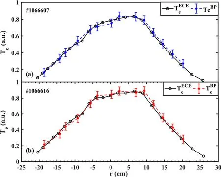
Figure 6.Prediction of average relative electron temperature profiles by different test sets, in shot (a) #1066607 and (b) #1066616.

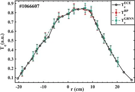
Figure 7.Comparison by two networks of BP NNs(red circles)and GRNN (green circles) to predict Te profile in shot #1066607.

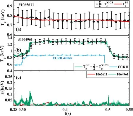
Figure 8.Prediction of core electron temperature obtained by XICS in shots (a) #1065611, (b) #1064961 and (c) their absolute errors.

On the J-TEXT,XICS measures the core absolute electron temperature,andcan also be predicted as similarly as the ECE signals.In the new model,the input parameters and hyperparameters are the same as those for the prediction ofwhileneandIsxrsignals in plasma core are used as input parameters, andas the training target (output parameters).All samples are from database B.Figure 8 shows the prediction of core absolute electron temperature in two shots without/with ECRH.In shot #1064961,Tejumps up during 0.32–0.49 s when the ECRH system turns on(figure 8(b)).The average errors without/with ECRH heating are less than 3%and 5%,respectively.The network can reproduce a significant increase ofTeto ～1.3 keV after the application of ECRH,and the recovery ofTeback to 0.8 keV at 0.53 s after removing ECRH.In addition to the steady stateTeprediction, the difference betweenandis larger during the transient state, i.e.during the increase (or decrease) ofTeat around 0.295 s(or 0.495 s).This might be due to the feature of XICS,which integrates the x-ray spectra for a few milliseconds and hence provides a time averagedTe(10 ms average in this shot).Future study using ECE as the target might reveal the fast variation ofTeduring the application of ECRH.

4.Summary and discussion

Electron temperature and its profile have been predicted by BP network and GRNN on the J-TEXT, based on basic plasma parameters, including plasma current, toroidal magnetic field,soft x-ray emission, electron density and loop voltage.The average error of the predictedTeis less than 5%, and MHD activities like sawtooth oscillations can be reproduced in the prediction.The network predicts electron temperature properly because it can fit the relation betweenTeand other signals.

This method can reduce the high reliability requirements of such diagnostic devices.The electron temperature may be predicted by sufficient diagnostic signals in real-time via adaptive neural network when there are enough diagnostic signals, if measurements ofTewas missing or lacked due to malfunction.In the future, the model ofTeprofile prediction will be improved from the current 14 networks to a single network, which although might increase computing power.

Acknowledgments

This work was supported by the National Magnetic Confinement Fusion Science Program (Nos.2018YFE0301104 and 2018YFE0301100), State Key Laboratory of Advanced Electromagnetic Engineering and Technology (No.AEET2020KF001) and National Natural Science Foundation of China (Nos.12075096 and 51821005).