Quench dynamics in 1D model with 3rd-nearest-neighbor hoppings?

Shuai Yue(岳帥), Xiang-Fa Zhou(周祥發(fā)),?, and Zheng-Wei Zhou(周正威),?

1Key Laboratory of Quantum Information,Chinese Academy of Sciences,Hefei 230026,China

2Department of Optics and Optical Engineering,University of Science and Technology of China,Hefei 230026,China

Keywords: Kibble–Zurek mechanism,Landau–Zener transition,topological defect,topological insulator

1. Introduction

Kibble–Zurek mechanism (KZM) describes the nonequilibrium dynamics and the formation of defects in a system when it quenches across the critical point of a continuous phase transition at a finite rate. Around the critical point, the relaxation time of the system increases, and adiabatically traversing this point becomes impossible. Employing adiabatic-impulse approximation, KZM can predict the defect density without solving complicated differential equations. The defect production during the quench follows universal scaling laws determined solely by the universality class of the underlying phase transition, which provides an elegant method to investigate phase transition dynamics. This theory has been widely applied and verified in many studies related to the early universe,[1]classical phase transitions,[2–5]transitions of liquid helium,[2,6,7]quantum phase transitions,[8–11]etc.[12–14]Especially for quantum transitions in a 1D lattice system without symmetry breaking,the defect density is often referred to as the transition probability to excited bands when the system initially occupies the lower energy band.[15–20]

Topological insulators have been a research hotspot in recent years.[21–25]In the most straightforward cases, they can be described by the standard band theory possessing unique topological properties.[21,22,24–27]Meanwhile, the non-trivial topology of the system can also result in many novel transport properties, which are still under active investigation. Due to their simplicity, 1D topological models are ideal platforms to investigate non-equilibrium dynamics. For instance,the KZM in Kitaev chain and Creutz ladder has been extensively considered where anomaly defect production rates are discussed after sweeping across a topological critical point.[17,28]In addition,the survival probabilities of edge Majorana fermions can even be used to distinguish different topological phases.[19,29,30]However, most of these investigations focus mainly on KZM in a 1D lattice model with only nearest-neighbor hopping.Physically,the presence of long-range hopping yields complex band structures with non-trivial topological properties. The system can exhibit richer dynamical behaviors,which deserve further investigation.

In this work,we consider a 1D lattice model with the 3rdnearest-neighbor hopping. The system supports topological phases carrying different invariants within different parameter ranges. KZM is explicitly considered in the cases of periodic boundary conditions (PBC) and open boundary conditions(OBC).For PBC,we find that the defect production for an initial bulk states can be well described by the standard KZM scaling law. For OBC, we find the oscillation of the defect production due to the interference of the edge modes and bulk states. In addition,both the bulk states and the edge modes support a path-dependent defect production rate,which violates the universal Kibble–Zurek scaling relation.

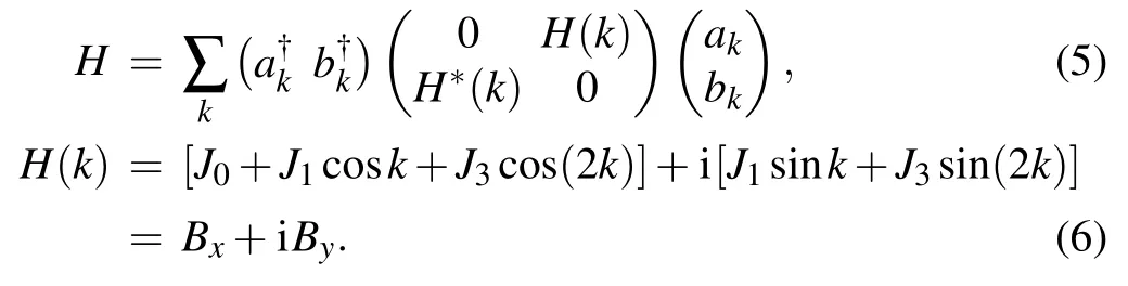
2. The model Hamiltonian

The model we consider is a modified bosonic Su–Schrieffer–Heeger model with alternative long-range hopping terms. The Hamiltonian reads

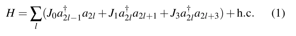
Fig.1. Diagram representation of Hamiltonian(1).

3. Quench dynamics in periodic boundary conditions

In the case of periodic boundaries, the system has space translational symmetry (STS). The Hamiltonian can then be block diagonalized in momentum space. To show this,we introduce a 2-component discrete Fourier transformation as

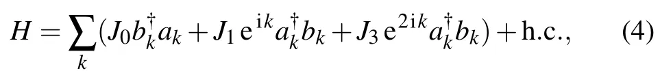
with the even positive integer N representing the number of lattices. Here the wave vector k is constrained in the first Brillouin zone, and reads kn=4πn/N with n=?N/4,?N/4+1,...,N/4?1. Substituting Eqs.(2)and(3)into Hamiltonian(1)yields

which can be rewritten as

Equation(5)indicates that the Hamiltonian is composed of N/2 pairs of decoupled 2-level systems for different kn.Eigen energies of the system can be obtained by solving its characteristic polynomial and reads

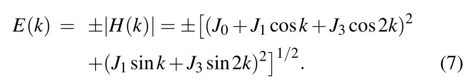
The system supports different topological phases. The boundaries between these phases can be determined by calculating the relevant excitation gaps,which disappears when

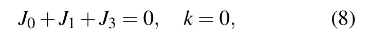
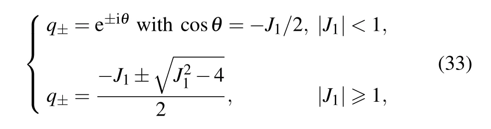
This leads to the phase diagram shown in Fig.2. For simplicity, in the sections below, we set J3=1. For different phases,we introduce the winding number defined as

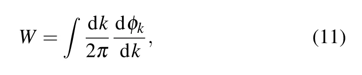
with φk=tan?1(By/Bx). Geometrically,W describes the total number of times the vector(Bx,By)travels counter-clockwise around the point (0,0). In our system, the corresponding winding numbers of the three topologically distinct phases denoted by I,II,and III are 1,2,and 0,respectively. According to bulk-boundary correspondence, this winding number is a topological invariant which equals the number of edge states on one end of the chain with open boundaries.

To illustrate the universal scaling law of KZM across the critical point, here we consider the transition line along with the hopping J1with fixed J0=?1 and J3=1. In this case,Eq.(7)yields

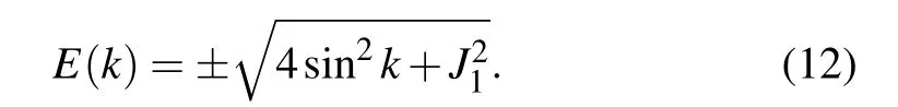
The energy spectrum is shown in Fig.2(b). Since different wave vector k can share the same Ek(see Eq. (12)), the relevant energy eigenstates are 4-fold degenerate.

For an initial bulk state in the lower band with fixed k,only the corresponding state in the upper band with the same k couples with it. Therefore,the system can be simplified into a set of decoupled two level systems. Equation(12)is exactly the same as the dispersion relation of Landau–Zener transition(LZT).Thus we can analytically calculate the evolution using LZ formalism[44–48](refer to Appendix A for details). The transition probability to the upper band for the eigenstate with kn=4nπ/N can then be obtained as

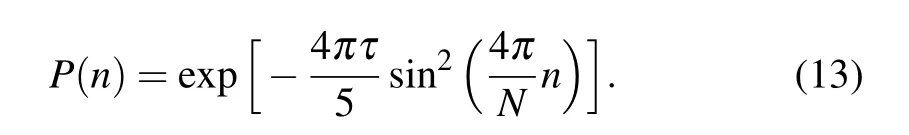
Therefore, if the initial state is the equal-weighted superposition of all eigenstates with negative energies,the defect density is

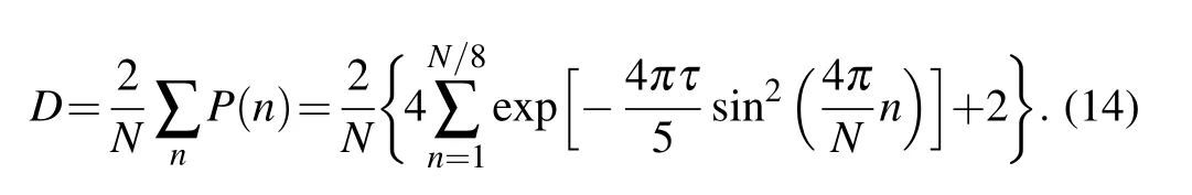
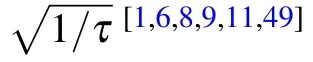
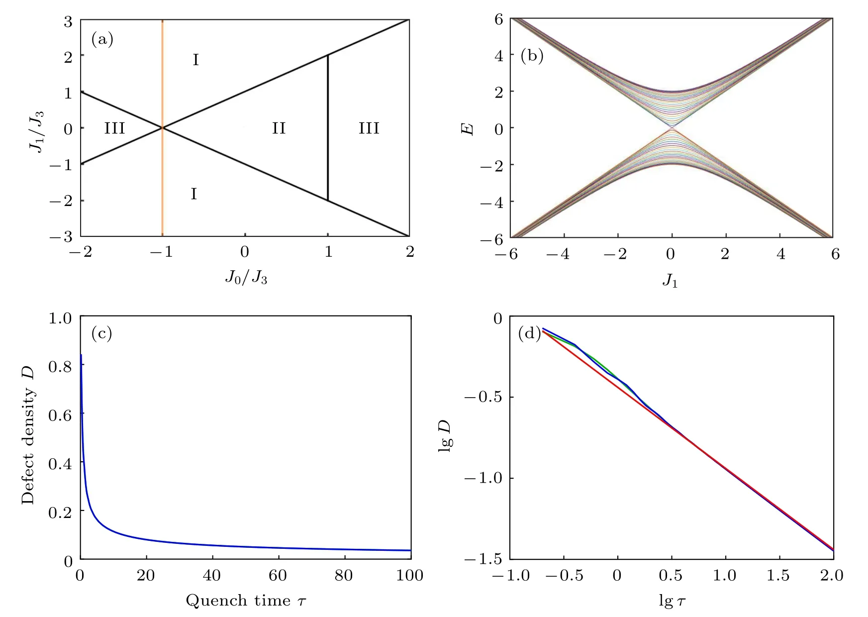
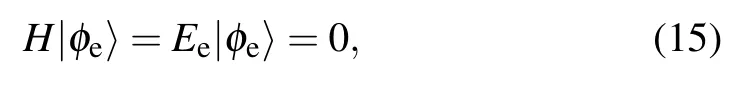
Fig.2. (a) Phase diagram of Hamiltonian (1) in J1–J0 plane. I, II, III represent different phases with the winding number 1, 2, and 0,respectively. The orange line is the quench path with fixed J0=?1. The initial and final positions are not shown since they are far away from the critical point. (b)The energy spectrum of Hamiltonian(1)with fixed J0=?1 and J3=1 in PBC.The number of lattice sites is set to be N=200. (c)Dependence of defect density on the quench time τ in PBC for a fixed quench rate J1=5t/τ (?τ ≤t ≤τ). The initial state is the equal-weighted superposition of all bulk states in the lower band. Here the green line is the defect density calculated through Eq.(14),the blue line is the numerical result. These two lines overlap with each other. (d)is the same result of(c)in common logarithmic coordinates. The red line is the KZ scaling ,which has a slope of ?1/2.

4. Quench dynamics in open boundary conditions

The system exhibits unusual behaviors in OBC. Due to bulk-boundary correspondence,different phase regions are divided by winding number and the degeneracy of edge states is 2 times of it. Analytical dynamics of the system can no longer be obtained easily due to the absence of STS. There exist complicated couplings between eigenstates. Especially for topological phases discussed here, the quench dynamical of the system also exhibits many new features due to the presence of edge modes. The production rate of the defect density also becomes very different from the usual KZ scaling.To show this,we start with the typical dynamical behavior of edge states.

4.1. Defect production of edge states

In OBC,the zero-energy edge states|φe〉are determined by

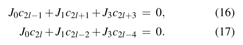
Since the odd and even sites are decoupled in or the even sector, depending on which ends it inhabits. In the odd sector,the coefficients clcan be obtained by solving the characteristic equation

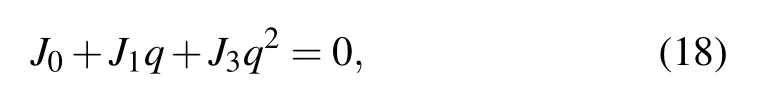
with the solution

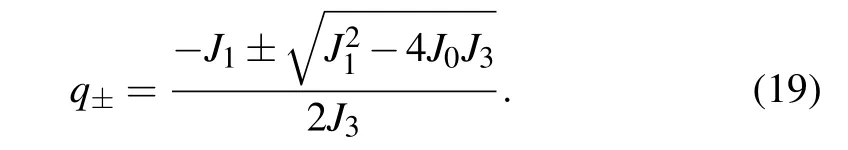
The general two linear independent zero modes can be written as

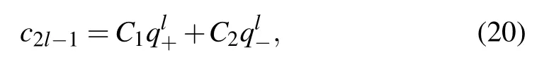
with C1and C2arbitrary constants. The existence of these edge modes can be analyzed by examining whether |q±| is larger than 1 or not,which is proved to be consistent with the discussion given by the winding number W. A similar discussion also applies to the even sector with two solutions defined as p±=1/q±. For instance,in the simplified case with J0=?1 and J3=1, we have|q+|>1>|q?|for J1＜0 and|q?|>1>|q+|for J1>0,the two edge modes then read

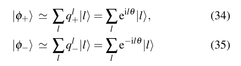
In Fig.3, we have plotted the defect density of the edge states along with the quench rate vq=5/τ. The initial state is set to be the equal superposition of the two edge modes. Since these modes inhabit different sectors of the chain,they decouple with each other in the adiabatic limit with longer quench time and merge into the bulk states in the upper or lower bands after across the critical point. However,in the case of the fast quench, the defect density D ～0, which confirms the above discussions.

In the intermediate regime with |J0|＜1, the above KZ dynamics can be viewed as the combination of quenching through two successive critical points. The presence of additional edge modes in phase II affects the evolution of the initial edge state. The dynamics is path-dependent and the density of defect shows very different behaviors,as will be discussed in detail in section 4.3. Especially when J0=0, the edge state is decoupled from the dynamics and remains unchanged for arbitrary quench rate vq.

Fig.3.(a)Energy spectrum of Hamiltonian(1)in OBC with J0=?1,J3=1 and N =200. (b) Dependence of defect density of edge states on quench time in OBC.Here the quench parameter reads J1=5t/τ with ?τ ≤t ≤τ.The initial state is the equal-weighted superposition of two edge states.

4.2. Oscillation of defect density induced by edge states

The presence of edge states can result in the oscillation of defect density. To show this,we consider the quench dynamics for J1=5t/τ (?τ ≤t ≤τ)with fixed J0=?1 and J3=1 in OBC.The spectrum of the system is shown in Fig.3(a). We also set the initial state as an equal-weighted superposition of all negative band eigenstates and 2 edge states,

Here |φm〉 represents the bulk eigenstate of the system with the wave vector km=4mπ/N for 1 ≤m ≤N/2 ?1. The two edge states are also denoted by |φm(?τ)〉 with m=N/2 and N/2+1,respectively.

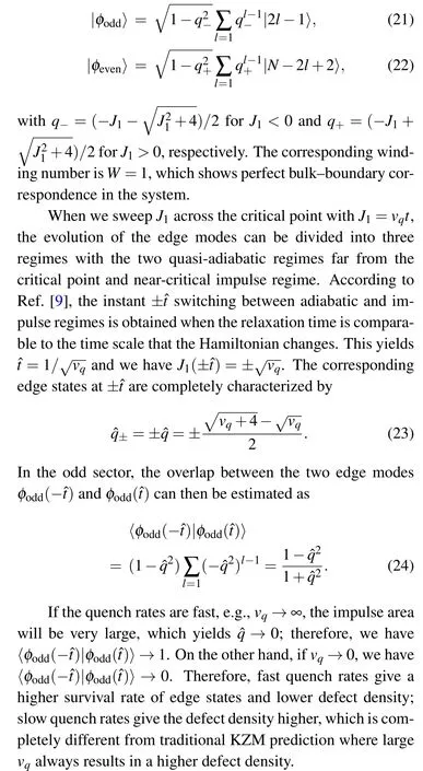
The defect density shown in Fig.4 exhibits an oscillation,which is caused by the interference of edge states and bulk states. Though analytical calculation is complicated in OBC,a good approximation to study such quench dynamics can be provided within the KZM paradigm. The evolution of our system quenching through the critical point can be divided into three regions,which are adiabatic,impulse,and adiabatic processes. The state of the system evolves adiabatically far away from the critical point and becomes “frozen” in the impulse region when getting close to the critical point.

Fig.4. (a)The oscillation of defect density caused by interference between bulk states and edge states. Other parameters are the same as those of Fig.3.The initial state is the equal-weighted superposition of all negative band eigenstates and 2 edge states. (b) is the defect density of (a) in common logarithmic coordinates. The slope of the red line is ?1/2.

where Emis the corresponding eigen-energy, cm(?τ) is the coefficients of the initial state, and γm(?τ,??t)represents the Berry phase defined by

According to Eq.(25), we have cm(?τ)=const/=0 for 1 ≤m ≤N/2+1,and cm(?τ)=0 for m>N/2+1. The geometric phase γmis always 0 since〈φm|φm〉=1 and〈φm|˙φm〉is real.

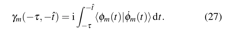
The evolution between ??t and ?t is considered to be“frozen”due to impulse approximation. Therefore the state of our system is redistributed at time ?t,and then evolves adiabatically again until the time τ. The oscillation period is closely related to the phase difference generated in the adiabatic regions. To illustrate this,we consider the dynamical evolution of the bulk part in Eq.(25). Within the KZM paradigm, the bulk part yields

Fig.5. The defect density for initial bulk states. The green line is the result(30)obtained form the KZM paradigm with β =32.11. The blue line is the numerical results. Other parameters are the same as those of Fig.3.

The last term above describes the interference within the upper band for the final wave function. Since the projected edge state|Edge+(τ)〉depends on phase θ,this results in the oscillation of defect density along with the quench time τ.Thus we can easily get the oscillation period T ?4π/5,which is clearly shown in Fig.4.

4.3. Defect production of quenching across phase regions

The presence of two non-trivial topological phases in the diagram allows us to explore many unusual dynamical behaviors of the system in the case of OBC. Physically, we can tune the hopping amplitudes along different paths, as shown in Fig.6(a). In these cases, the system sweeps across phase II (W =2) along different lines with two successive critical points or a critical line. The defect density reveals very complicated couplings in OBC, as we will show in detail below.Similar to the last subsection, we set the initial states as the equal-weighted superposition of all bulk states in the negative band and all existing edge states.

In Figs.6(c)and 6(d),we have plotted the calculated result for the quench line with fixed J0=0 and J3=1. The system sweeps across phase regions I,II,I for J1=5t/τ with?τ ≤t ≤τ,as shown in Fig.6. One can see that in this case,the oscillation in the defect production disappears,and no defect is excited for initial edge modes for all τ. This indicates that the edge states in region I are also decoupled from those bulk states and new edge modes in phase II. Further analysis shows that in this case,the characteristic ratio q=0 is always possible when J0=0,which yields the edge states|φodd〉=|1〉and |φeven〉=|N〉 for arbitrary J1. When J0=0, these two states are decoupled from other lattice sites. Therefore, the initial edge states in region I do not contribute to the defect density.

For fixed J0=1 and J3=1,our system quenches across the boundary between phase regions I and II, as shown in Fig.6(a). In this case,we have a 1D gapless surface instead of a gapless point around J1～0. In the case of PBC,the defect density D for initial bulk states in the lower band is always 1 even in the adiabatic limit. This can be understood as in the intermediate regime around J1～0, the two bands are completely decoupled. Therefore, after sweep across the critical regime, the roles of the two bands are interchanged, and all the initial bulk states are excited.

However, for open boundaries, bulk states in the two bands can couple with each other around the gapless point k=kcdescribed by coskc=?J1/2 in the momentum space.This can be shown by considering the explicit form of the edge states. In this case,the solution of characteristic Eq.(18)reads

When|J1|≥1 within the regime I,only one of|q+|and|q?| has module less than 1, which characterizes the wavefunction of edge mode. At the critical point|J1|=1,we have|q±|=1. The two edge modes in the regime|J1|＜1 can then be written as

Edge modes along the critical line can then be written as the combinations of gapless bulk states

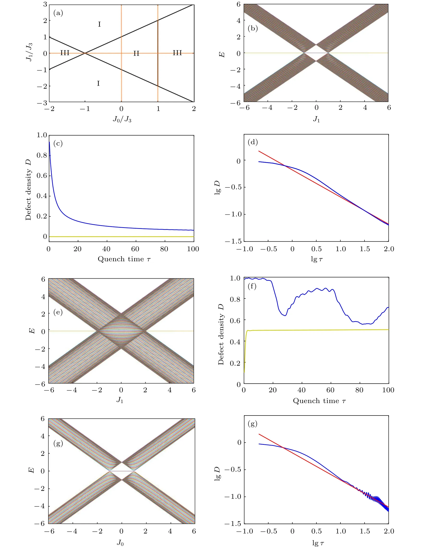
Fig.6. (a) Different quench paths shown in the phase diagram. (b) The spectrum of Hamiltonian (1) as a function of J1 with N =200,J0=0,and J3=1 in OBC.(c)shows the dependence of defect density on quench time τ in OBC with J1=5t/τ (?τ ≤t ≤τ). The initial state is the equal-weighted superposition of all bulk states in the negative band and 2 edge states. (d)is the dependence of(c)in common logarithmic coordinates, the slope of red line is ?1/2. The yellow line in(c)is the defect density for initial edge states. The conditions of(e)and(f)are the same as(b)and(c)except for fixed J0 =1. (g)The spectrum of Hamiltonian(1)as a function of J0 with N =200,J1=0,and J3=1 in OBC.(h)shows the dependence of defect density on quench time τ in OBC with J0=5t/τ (?τ ≤t ≤τ). It is plotted in common logarithmic coordinates and the slope of red line is ?1/2. The initial state is the equal-weighted superposition of all bulk states in the negative band.

This indicates that edge states are linked with the different bulk states carrying the characteristic momentum kcwithin the regime 1 ≥J1≥?1. Therefore,any initial edge state becomes completely delocalized when we sweep across the critical line adiabatically. Meanwhile, when the initial state is set to be the superposition of the edge modes and the bulk states in the lower band, the complicated coupling between those eigenstates within the critical regime also results in the unusual oscillation behavior of the defect density for different quench time τ,as shown in Fig.6(f)(see blue line in the panel).

For fixed J1=0 and J3=1, our system sweeps across phase regions III, II, III, whose winding numbers are 0, 2, 0,respectively.Although the initial state is pure bulk and no edge states are involved, the oscillation of D still exists, as shown in Fig.6(h). This is because that in the intermediate regime around J1=0,the system is driven to be a complicated superposition of different eigenstates. Therefore,the edge modes in phase II are not empty occupied in OBC,which thus results in the oscillation of the defect D for longer quench time τ.

5. Conclusion and outlook

To summarize,we have studied the quench dynamics of a 1D topological model with 3rd-nearest-neighbor hopping using both analytical and numerical methods. In PBC,we found that the defect density obeys the universal KZ scaling law when the system sweeps across the critical point. For OBC,the presence of edge modes results in many unusual dynamical features. We showed that the survival probability of the edge states could be much larger for fast quench and vanishes in the adiabatic limit. We also found the oscillation of the defect density due to the interference of edge and bulk states. In addition,the scaling law of defect production depends closely on specific quench paths,which does not follow the usual scaling law predicted by KZM.There are still open problems worthy of further investigations, such as the defect production of quench dynamics with dissipation or in higher dimensional systems, the interference of edge states and bulk states under other conditions,etc. We believe that both the answers to the above questions and the results of the current work should be valuable for understanding the unusual dynamics in the lattice system with non-trivial topology.

Appendix A: Dispersion relation of Landau–Zener transition

For a 2-level system with the following Hamiltonian

LZF provides the solution to dynamical equations of this system under certain conditions. Those conditions are referred to as Landau–Zener approximations, which are summarized as follows:

1. The perturbation parameter, i.e., diagonal elements H11=F1t and H22=F2t,in the Hamiltonian is a known,linear function of time.

2. The energy separation of the diabatic states varies linearly with time,namely,H11?H22=(F1?F2)t=2αt.

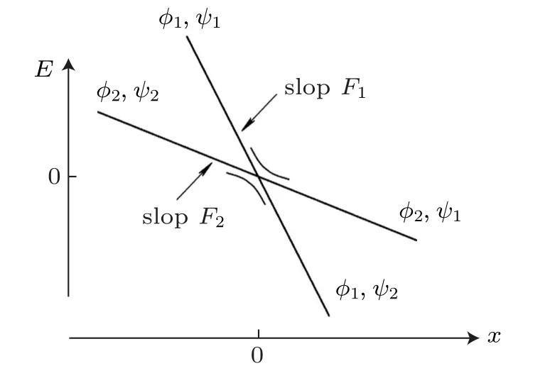
Fig.A1. The spectrum of the 2-level system under Landau–Zener approximations. φ1,2 are the diabatic basis,ψ1,2 are eigenstates of the Hamiltonian.

Figure A1 is the spectrum of the 2-level system. With these approximations, the differential equations of LZT can be solved analytically,yielding LZF as[48]

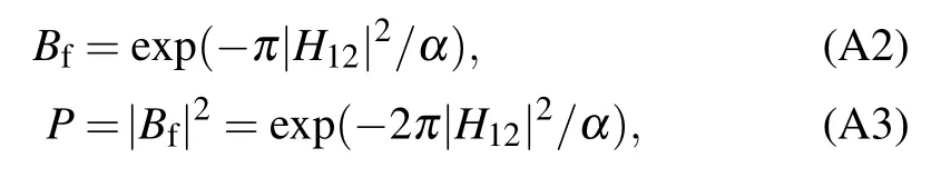
where Bfis the final coefficient of the basis vector of the upper band, H12is the coupling in the Hamiltonian matrix, and α is the rate of change of the energy separation. The dispersion relation(A1)in LZT is exactly the same as Eq.(12)and reads

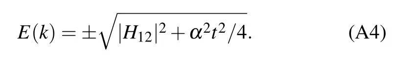
with kn=4nπ/N.

Appendix B:KZ scaling of Hamiltonian(1)

The defect density of a d-dimensional system quenching through an m-dimensional gapless surface is[1,6,8,9,11,49]

where ν is the critical exponent, z is the dynamic exponent which relates spatial with temporal critical fluctuations. This KZ scaling can be observed in our system with quantum transitions. For the two quench paths shown in Fig.B1(a), their defect densities scale as τ?1/2and τ0,respectively. We calculate the defect densities in PBC numerically in Fig.B1(b),and the results fit KZ scaling quite well.

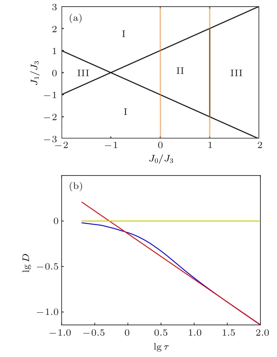
Fig.B1. (a) The two quench paths we proposed to verify the scaling law.The left red line takes a fixed J0 =0, and the right one has a fixed J0 =1.They quench through a 0-dimensional transition point,or a one-dimensional gapless surface, respectively. (b) The dependence of defect density on quench time in common logarithmic coordinates in PBC.Other parameters are set to be N =200, J3 =1, and J1 =5t/τ with ?τ ≤t ≤τ for a fixed quench rate. The blue line represents the dependence of the defect density along with the quench rate for J0 =0, and the yellow line is the case with J0=1. In both cases,the initial states are set to be an equal-weighted superposition of all bulk states in the negative band. The slope of the red line is?1/2.