ON BLOW-UP PHENOMENON OF THE SOLUTION TO SOME WAVE-HARTREE EQUATION IN d ≥ 5*
2020-08-03 12:06:02SuxiaXIA夏素霞
Suxia XIA (夏素霞)
College of Science, Henan University of Technology, Henan 450001, China
E-mail: xsx0122@126.com
Abstract This article mainly considers the blow up phenomenon of the solution to the wave-hartree equation utt ? △u = (|x|?4 ? |u|2)u in the energy space for high dimensions d ≥ 5. The main result of this article is that: if the initial data (u0, u1) satisfy the conditions E(u0, u1) E(W, 0) and for some ground state W, then the corresponding solution must blows up in finite time.
Key words Cauchy problem; wave-hartree equation; blow up; Strichartz estimate
1 Introduction
has been also studied by many authors(see[6,8,15,17–21,25–28]and references therein). For the subcritical cases in the defocusing case,Ginibre and Velo[6]derived the associated Morawetz inequality and extracted a useful Birman-Solomjak type estimate to obtain the asymptotic completeness in the energy space. Nakanishi [7] improved the results by a new Morawetz estimate which does not depend on the nonlinearity. For the critical case,Miao, Xu, and Zhao[8]took advantage of a new kind of the localized Morawetz estimate,which is also independent of the nonlinearity,to rule out the possibility of the energy concentration at origin and established the scattering results in the energy space for the radial data in dimension d ≥5. For the general data and focusing case,please refer to[17–21]. For the blow up solutions of the fractional Hartree equation, please see [25, 26, 28].
Before stating our main result, we introduce some notations. Let(Rd)×L2(Rd) be the energy space, and the energy be defined as

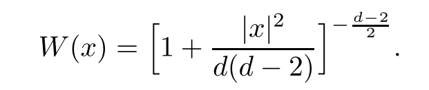
Definition 1.1Let W(x) be the ground state of the elliptic equation
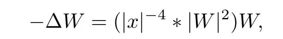
and the exsitence and uniqueness of the ground state was proved in [9].
The main result of this article is
Theorem 1.2Suppose thatsatisfy

and let u be the corresponding solution to (1.1) with maximal interval of existence I =(?T?(u0,u1),T+(u0,u1)). Then, u blows up both forward and backward in finite time, that is,T?(u0,u1),T+(u0,u1)<+∞.
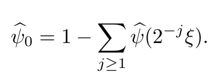
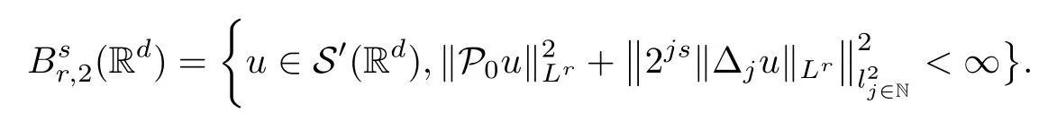
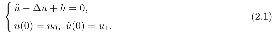
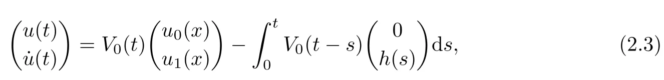
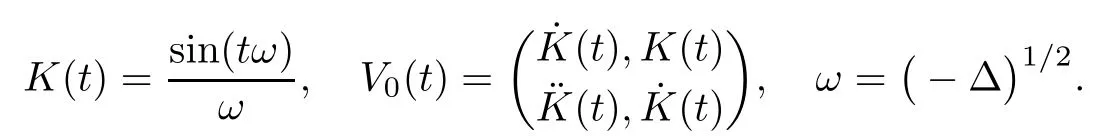
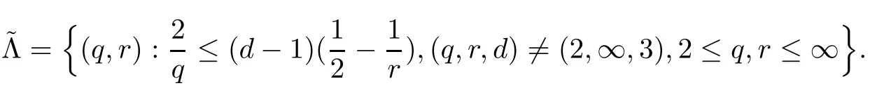
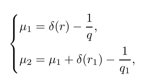
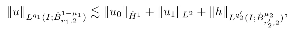
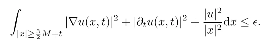
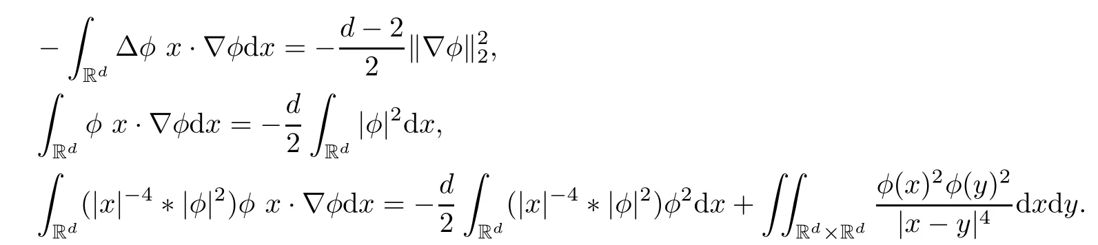
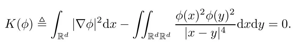
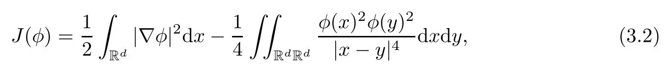
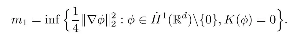
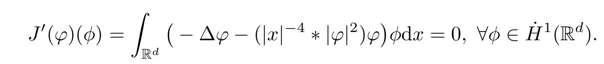
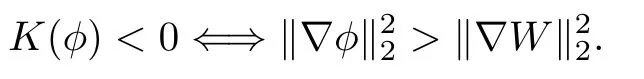
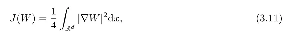
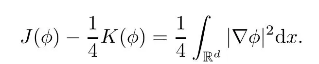
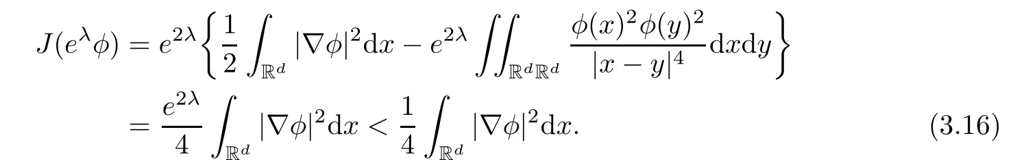
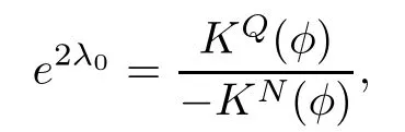
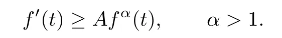
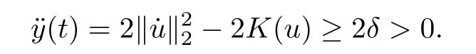
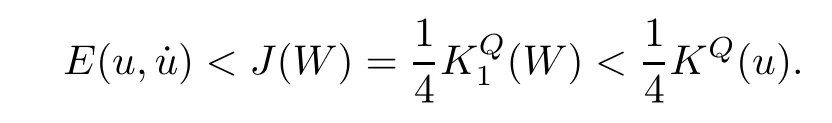
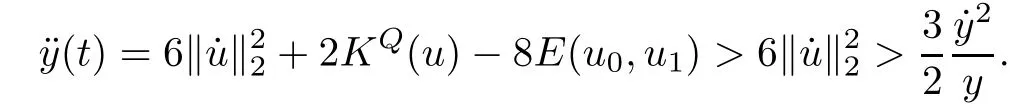
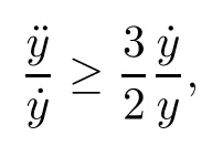
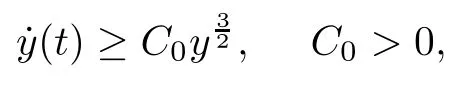
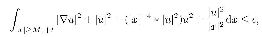
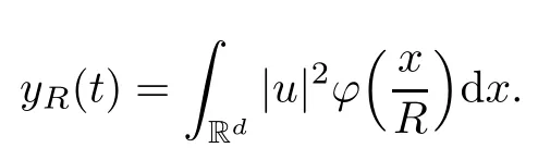
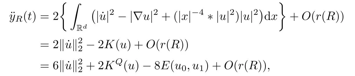
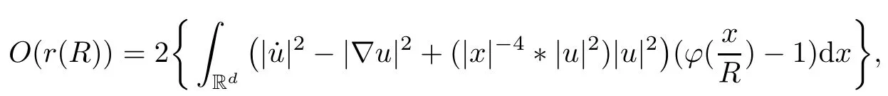
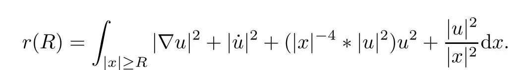
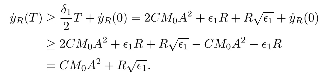
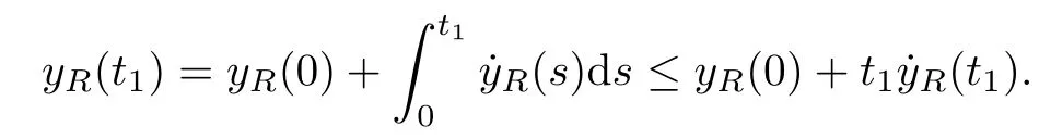
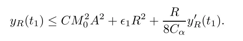
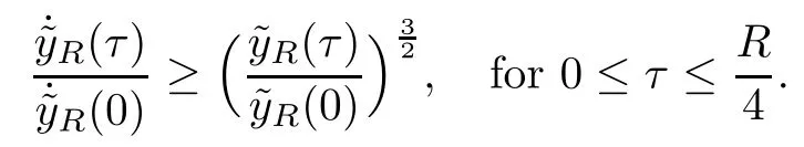
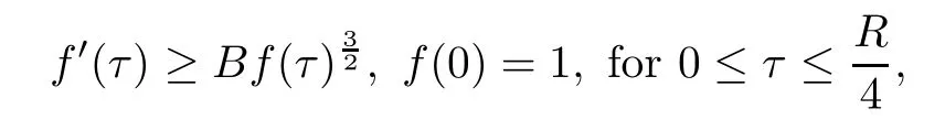
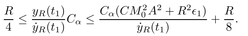
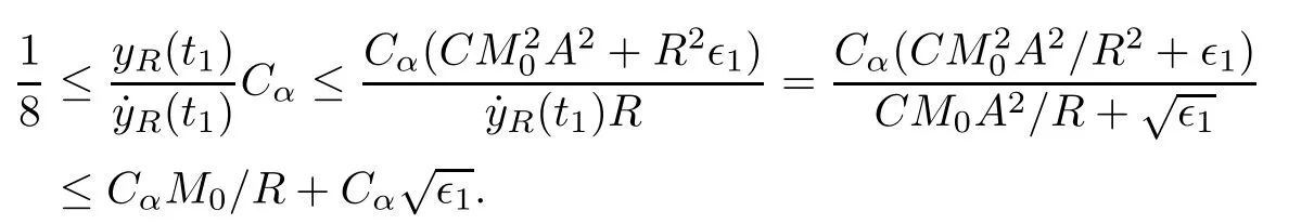
Remark 1.3It follows from Lemma 3.7 below that the restrictionis equivalent to the restrtictionunder the assumption E(u0,u1) One may resort to the causality(Lemma 4.1 in Menzala-Strauss[3]), however it holds only for the case V ∈Ld/3+L∞, which does not contain the critical cases, and the exponent d/3 stems from the estimate of the term ∫ut(V ?u2)udx as we know that it cannot be controlled by the energy if V ∈Lpwhen p<.To overcome it,we make use of the finite speed of propagation of the free operators K(t)and ˙K(t)and the boundness of the local-in-time Strichartz estimate of the solution(the nonlinear interaction is actually the linear feedback),to establish the causality for critical cases V ∈Ld4+L∞. See the details in Section 2. In fact, we can establish the causality for all subcritical cases. Here, we only need the critical cases. This article is organized as follows. In Section 2, first we recall the Strichartz estimates for equation(1.1),and then establish the extended causality. In Section 3,we discuss the property of the ground state. In Section 4, we prove Theorem 1.2. Finally, we conclude the introduction by giving some notations which will be used throughout this article. We always assume the spatial dimension d ≥3 and let 2?=. For any r,1 ≤r ≤∞, we denote bythe norm in Lr= Lr(Rd) and by r′the conjugate exponent defined by= 1. For any s ∈R, we denote by Hs(Rd) the usual Sobolev spaces. Let ψ ∈S(Rd) be such that suppand Define ψ0by For any interval I ?R and any Banach space X, we denote by C(I;X) the space of strongly continuous functions from I to X and by Lq(I;X) the space of strongly measurable functions from I to X withGiven d, we define, for 2 ≤r ≤∞, Sometimes abbreviate δ(r), δ(ri) to δ, δirespectively. We denote by<·,·>the scalar product in L2. In this section, first we give some Strichartz estimates. Consider the Cauchy problem for the following linear equation The integral equation for the Cauchy Problem (2.1) can be written as or where Let U(t)=eitω, then Lemma 2.1Let (q,r),(q1,r1)∈, and Then, where Corollary 2.2Let d ≥5, u ∈C(I;) be a strong solution of (1.1), then Now, we state the local well-posedness for (1.1) with large initial data. Define Theorem 2.3(LWP) Assume that d ≥5, (u0,u1) ∈×L2, 0 ∈I an interval, andthen there exists δ =δ(A) such that if there exists a unique solution u to (1.1)in I×Rd, with (u, ˙u)∈C(I;×L2), and ProofWe apply the Banach fixed point argument to prove this lemma. First, we define the solution map on the complete metric space B It suffices to prove that the operator defined by the RHS of (2.5) is a contraction map on B for I. In fact, by Lemma 2.1, we have From the fractional Leibnitz rule and the H?lder and Young inequalities, we get By the interpolation, one has Plugging (2.7) into (2.6), and u ∈B, we obtain provided that On the other hand, by a similar argument as before, we have, for ?ω1,ω2∈B, which allows us to derive by taking δ small such that A standard fixed point argument gives a unique solution u of (1.1) on I which satisfies the bound (2.4). Next, we recall the causality. Lemma 2.4(Extended Causality, [10]) Assume that (u0,u1)∈×L2satisfy for some constant R>0 and u(t)is the finite energy solution to equation(1.1)with initial data u0,u1. Then, it holds that By the Strichartz estimates and the causality,we can obtain the following lemma as Lemma 2.17 in [11]. Lemma 2.5Letwith maximal interval of existence I = (?T?(u0,u1),T+(u0,u1)). There exists ?0> 0 such that, if for some M =M(?)>0 and 0 ProofOne may refer to [11] for details of the proof. In this section, we prove existence of ground state as another constrained minimizers, and some preliminary lemmas for the study in the focusing case. The idea is similar to S.Ibrahim,N.Masmoudi, and K.Nakanishi [12]. First, by direct computation, we have the following Pohozaev identities: Lemma 3.1Assume φ ∈S(Rd), then Lemma 3.2Let φ be the ˙H1(Rd) solution of the following equation then there holds ProofMultiplying (3.1) with φ in both sides and integrating. Let the static energy J be defined by We also define The existence and uniqueness of the ground state has been shown in[9], and denoted by W(x). Lemma 3.3Let, and Before proving Lemma 3.3, we recall some notations and two important lemmas in [12].First, we decompose K() into the quadratic and nonlinear parts: Remark 3.4Clearly, there holdsas λ →?∞. Lemma 3.5For any bounded sequencesuch that, we have, for large n, ProofUsing the H?lder and Young inequality, we have Plugging (3.6) into (3.5), we obtain Lemma 3.6If set, and then m1=m. Moreover m=J(Λ). Proof Step 1m1=m. It is trivial to prove that m1≤m becauseif, so it suffices to show m ≤m1. Takesuch that K(φ)<0. and so Hence m ≤m1. Step 2m=J(Λ). By the(Rd) scale invariance and Step 1, we have By the homogeneity and the scaling, it is equal to where C denotes the best constant for the Sobolev inequality which is well-known to be attained by the following explicit W ∈(Rd) (see [9, 16]) Proof of Lemma 3.3From Lemma 3.6, we know that. So, it suffices to prove Λ1= Λ. Suppose ? ∈Λ, then it is easy to see that J(?) ≥m by the definition. Suppose ? ∈Λ1. As ? is a minimizer for (3.3), there exists a Lagrange multiplier η ∈R such that and so η =0. Hence, J′(?)=0, namely, So, ? satisfies the elliptic equation: ??? ?(|x|?4?|?|2)? = 0. Therefore, m ≥J(?). Hence,m=J(?), which completes the proof of Lemma 3.3. The following lemma gives an equivalent description of the functional K(u) under the restriction of E(u0,u1) Lemma 3.7Assumesuch that J() ProofIt is easy to see that and Next, we prove the reverse statement. Noting if we take λ ∈R such that While by (3.14) and the assumption in Lemma 3.7, we obtain Combining this with (3.15), we have, which concludes the proof. As a consequence of Lemma 3.3, we deduce that the sign of K(u) is invariant along the flow of NLW under the restriction of E(u, ˙u) Corollary 3.8Let then A is invariant under the flow of NLW. That is, if (u0,u1) ∈A, then (u(t),∈A, for any t ∈(?T?(u0,u1),T+(u0,u1)). ProofAs J(u(t)) < E(u(t),,J(W) = E(W,0), and E(u(t),= E(u0,u1), we deduce that if E(u0,u1) < E(W,0), then there holds J(u) < J(W), for any t ∈(?T?(u0,u1),T+(u0,u1)). On the other hand, if there exists t ∈(?T?(u0,u1),T+(u0,u1)) such that K(u(t)) = 0,then by Lemma 3.3, we get J(u(t))≥J(W), which contradicts with J(u) By Lemma 3.7, one may replace A by The next Lemma gives a upper bound on K under the threshold m,which will be important for the blow up. Lemma 3.9Suppose that(Rd), J() ProofLet j(λ)=J(eλφ), then it follows from direct computation that and so j′(0)=K(), j′′(λ)<2j′(λ). If we choose λ0∈R such that then j′(λ0)=K()=0, and λ0<0 by K()<0. Therefore, we have which completes the proof. In this section,we prove Theorem 1.2 by the argument as in[11]. First,we give the following lemma Lemma 4.1Suppose the differential function f(t)≥0, and f(0)=1 satisfies Then, there holds where Cαis a constant depending on α. Proof of Theorem 1.2 Case 1u0∈∩L2. In this case,we assume that the initial data enjoys more regularity,that is, u0∈L2, which simplies the proof and gives some idea for the general case u0∈.The idea is essentially from Payne-Sattinger[24],but we give a complete proof for convenience. By contradiction we assume that the solution u exists for all t >0. The proof for t <0 is the same. It follows from Lemma 3.9 that there exists δ >0 such that K(u) Therefore, using Cauchy-Schwartz inequality and (4.1), we obtain, for any t>t0, Hence, for t>t0, we have which implies that, for t>t0, which leads to finite time blow-up of y(t). Case 2For general initial data u0. The idea comes from[11]. By contradiction we assume that the solution u exists for all t>0, that is, T+(u0,u1)=+∞. where and Arguing as in the proof of Case 1,let δ1=2KQ(u)?8E(u, ˙u),then it follows from the conditions of Theorem 1.2 that δ1>0. Hence, Now, choose ?1≤small enough and M0=M0(?1), such that and then for R>2M0, we have O(r(R))≤. Noting also that Thus,there exists 0 Now, we estimate T. We first choose ?1so small that, where Cαis the constant defined in Lemma 4.1 and R so large that,then we have(we can also ensure T ≤). Thus, If we now use the argument in the proof of Case 1, for the function, in light of, we see that for, we have then it follows from Lemma 4.1 that the time of blow-up for f is τ?with τ?≤CαB?1. Thus,we must have Thus, we have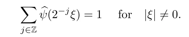
2 Preliminaries
2.1 Strichartz estimate


3 Variational Characterizations


4 Blow up


 Acta Mathematica Scientia(English Series)2020年3期