GLOBAL SOLUTION TO 1D MODEL OF A COMPRESSIBLE VISCOUS MICROPOLAR HEAT-CONDUCTING FLUID WITH A FREE BOUNDARY?
2017-01-21 05:29:58NerminaMUJAKOVI
Nermina MUJAKOVI′C
Department of Mathematics,University of Rijeka,Radmile Matejˇci′c 2,Rijeka 51000,Croatia
NelidaˇCRNJARI′C-ˇZIC
Section of Applied Mathematics,Faculty of Engineering,University of Rijeka,Vukovarska 58, Rijeka 51000,Croatia
GLOBAL SOLUTION TO 1D MODEL OF A COMPRESSIBLE VISCOUS MICROPOLAR HEAT-CONDUCTING FLUID WITH A FREE BOUNDARY?
Nermina MUJAKOVI′C
Department of Mathematics,University of Rijeka,Radmile Matejˇci′c 2,Rijeka 51000,Croatia
E-mail:nmujakovic@math.uniri.hr
NelidaˇCRNJARI′C-ˇZIC
Section of Applied Mathematics,Faculty of Engineering,University of Rijeka,Vukovarska 58, Rijeka 51000,Croatia
E-mail:nelida@riteh.hr
In this paper we consider the nonstationary 1D fow of the compressible viscous and heat-conducting micropolar fuid,assuming that it is in the thermodynamically sense perfect and polytropic.The fuid is between a static solid wall and a free boundary connected to a vacuum state.We take the homogeneous boundary conditions for velocity,microrotation and heat fux on the solid border and that the normal stress,heat fux and microrotation are equal to zero on the free boundary.The proof of the global existence of the solution is based on a limit procedure.We defne the fnite diference approximate equations system and construct the sequence of approximate solutions that converges to the solution of our problem globally in time.
micropolar fuid fow;initial-boundary value problem;free boundary;fnite diference approximations;strong and weak convergence
2010 MR Subject Classifcation35Q35;76M20;65M06;76N99
1 Introduction
This paper analyzes the compressible fow of the isotropic,viscous and heat conducting micropolar fuid,which is in the thermodynamical sense perfect and polytropic.The model for this type of fow was frst considered by Mujakovi′c in[1]where she developed a one-dimensional model.In the same work,the local existence and the uniqueness of the solution,which is called generalized,for our model with the homogeneous boundary conditions for velocity,microrotation and heat fux were proved.In the proof of this result the Faedo-Galerkin method was used. In the articles[2]and[3]the same method was used to prove the local existence theorems.
In this paper we consider the problem for the same fuid placed between a static solid wall and a free boundary connected to a vacuum state.We set up our problem frst in the Euler variables(y,t).Let at the initial moment t=0 fuid occupy a bounded domain[0,L]. Let the left boundary y=0 be an impermeable solid wall and the right one y=y0(t)be a boundary where fuid contacts with vacuum and be unknown in advance.We also assume the homogeneous boundary conditions for velocity,microrotation and heat fux on the fxed border and the homogeneous boundary conditions for the strain,microrotation and heat fux on the free boundary.Under the transition to the Lagrange coordinates(x,t)(see[1])we get the same boundary conditions at the borders x=0 and x=1.Here we prove the global existence of the solution for the described problem.In the proof,we do not use as in[1],[2]and[3]the Faedo-Galerkin method,which is not applicable to this type of problem.We use the fnite diference method instead.We applied the same method in[4]where the existence of global solution for the problem with homogeneous boundary conditions,defned in[1],was proved. In this paper the proof of the global solution is based on a similar procedure as in[4].Unlike in[4],where the positive lower and upper bounds for mass density existed,the main difculty here was the nonexistence of the positive lower bound for the mass density due to the assumed free boundary condition.As a consequence of that,in this paper more complicated estimating procedure than in[4],was necessary.
Let notice that in all previous research it was enough to assume that the initial density belongs to H1(h0,1i).In order to obtain more precise estimates,we propose here that it belongs to H2(h0,1i).In this paper we use some ideas from[5]where a similar method was used to prove the existence of the global solution for the classical fuid fow problem with spherical symmetry.However,the microrotation velocity that appears in our model causes additional difculties in investigating the existence of the solution for the considered problem.
In our work,the proof is based on a limit procedure.We defne the fnite diference approximate equations system,investigate the properties of the sequence of the approximate solutions and prove that the limit of this sequence is the solution to our problem on the domain (0,1)×(0,T),where T>0 is arbitrary.We follow some ideas of[6,7]also.
The paper is organized as follows.In Section 2 we introduce the mathematical formulation of our problem.In Section 3 we derive the fnite diference approximate equations system and in the fourth section present the main result.In Sections 5–8,we prove uniform a priori estimates for the approximate solutions.Finally,the proof of convergence of a sequence of approximate solutions to a solution of our problem is given in the ninth section.
2 Mathematical Model
We are dealing with the one-dimensional fow of the compressible viscous and heat-conducting micropolar fuid fow,which is thermodynamically perfect and polytropic.Let ρ,v,w and θ denote,respectively,the mass density,velocity,microrotation velocity and temperature in the Lagrangian description.The motion of the fuid under consideration is described by the following system of four equations(see[1]):
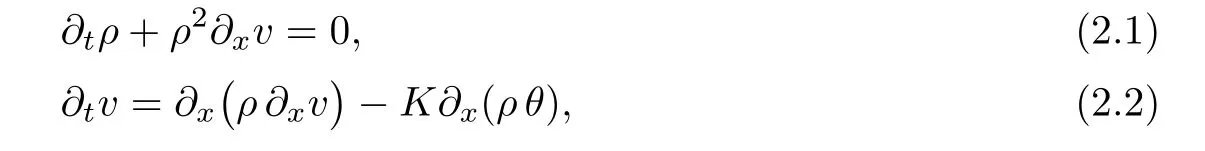
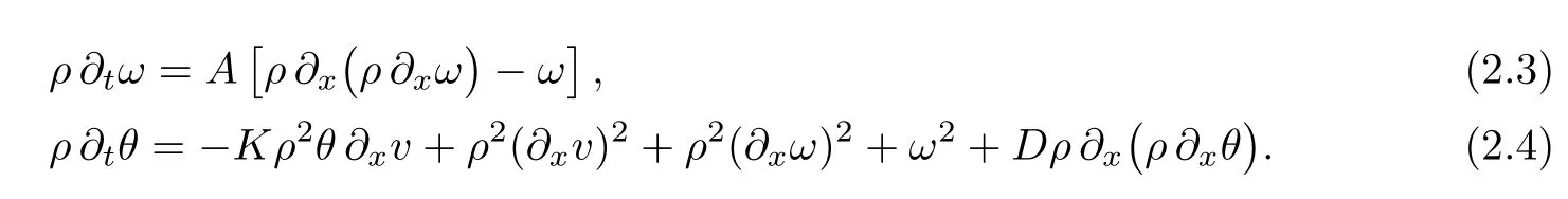
The system is considered in the domain QT=h0,1i×h0,Ti,where T>0 is arbitrary;K, A and D are positive constants.Equations(2.1)–(2.4)are,respectively,local forms of the conservation laws for the mass,momentum,momentum moment and energy.We take the following non-homogeneous initial conditions

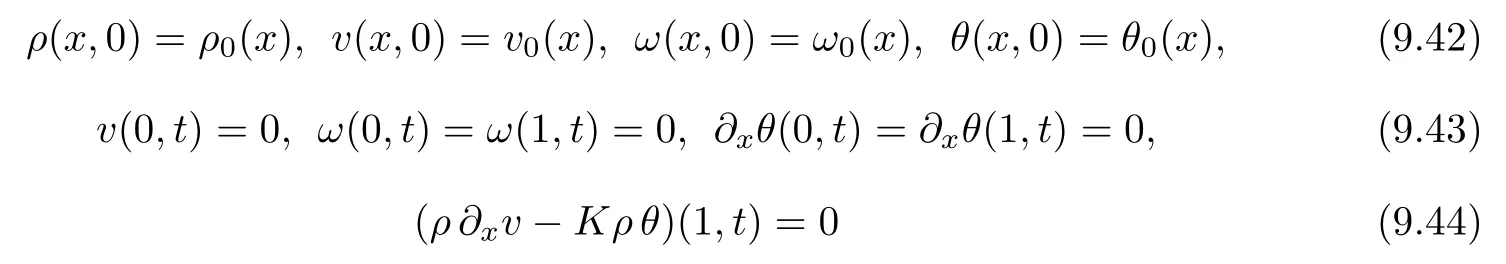
for x∈h0,1i.Here ρ0,v0,ω0and θ0are given functions.The solid boundary conditions and free boundary conditions are

for t∈h0,Ti.Condition(2.7)means that the strain equals zero on the boundary x=1.To articulate the assumption that there is no initial cavity with the fuid residing in the bounded region,we assume that there exists a decreasing non-negative function Λ:[0,1]→R+and a constant C0>0 such that
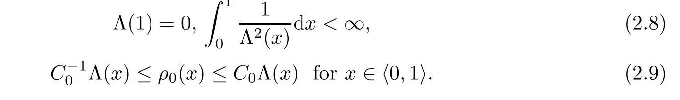
We assume

and that there exists a constant m∈R+such that

Let the initial data(2.5)have the following properties of smoothness

Because of the embedding Hk(h0,1i)into Ck?1([0,1])(e.g.[10,11]),it is easy to check that there exists M∈R+such that

3 Finite-diference Spatial Discretization and Approximate Solutions
In the similar way as in[4],in this section we introduce a space discrete diference scheme in order to obtain an appropriate approximate system of the equation system(2.1)–(2.7).We construct semidiscrete fnite diference approximate solutions on a uniform staggered grid.In making a discrete scheme we use some ideas from[5]and[6]also.
Let h be an increment in x such that Nh=1 for N∈Z+.The staggered grid points are denoted with xk=kh,k∈{0,1,···,N}and xj=jh,j∈?12,···,N?12?.For each integer N,we construct the following time dependent functions


that form a discrete approximation to the solution at defned grid points
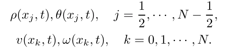
First,the functions ρj(t),vk(t),ωk(t),θj(t),j=12,···,N?12,k=1,···,N?1,are determined by using appropriate spatial discretization of the equation system(2.1)–(2.4):

where j=12,···,N?12and k=1,···,N?1,δ is the operator defned with

for l=j or l=k.For k∈{1,···,N}and j∈{12,···,N?12},the functions ρk,θkand vj,ωjwe defne by

Equations(3.3)–(3.6)are ordinary diferential equations.
Taking into account the boundary conditions(2.6)–(2.7),we defne

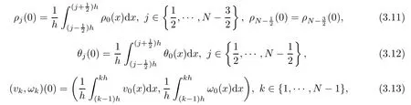
Condition(3.10)determines vN(t).Now the system(3.3)–(3.6)with(3.9)–(3.10)contains 4N+2 equations for 4N+2 unknown functions.The corresponding initial conditions are defned by the initial functions(2.5)as:
and

It is easy to see that from(2.9),(2.10),(2.11)and(3.15)it follows

for j=12,···,N?12and

Taking into account(2.8),(2.9),(2.12)and(3.16),one can conclude that
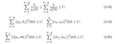
and
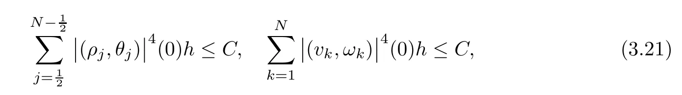
where C>0 is a constant,which depends on the initial functions and not on the step h(or N).
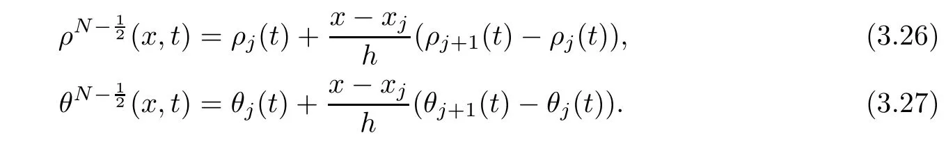
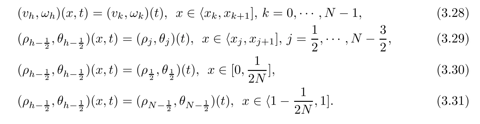
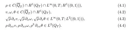
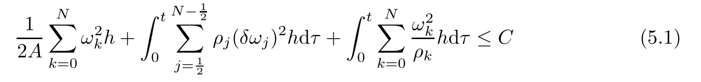
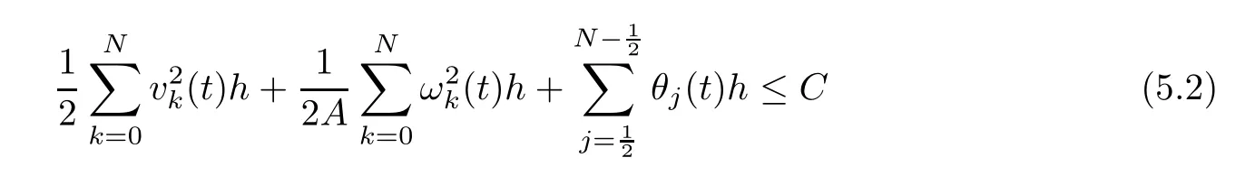
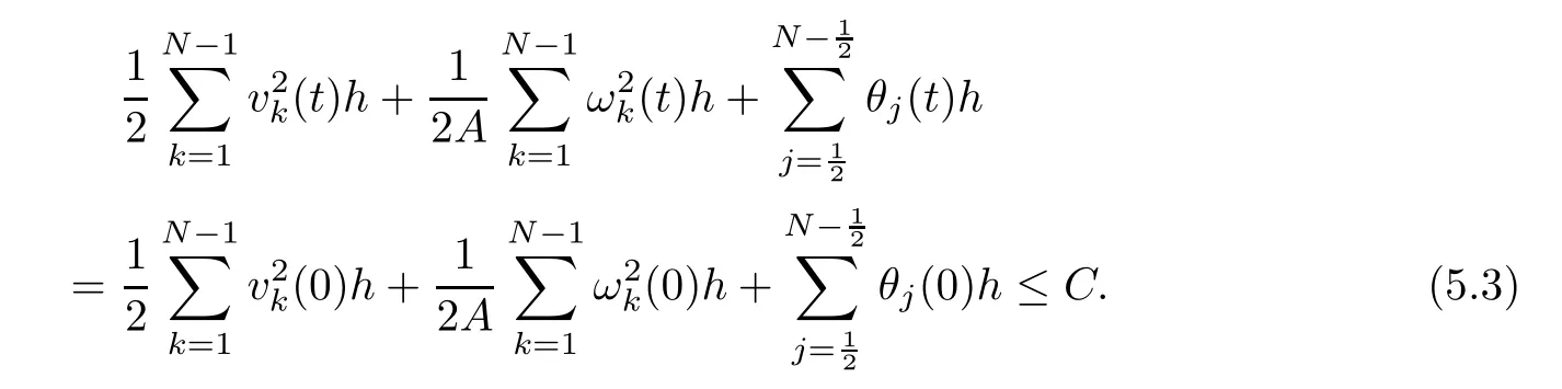
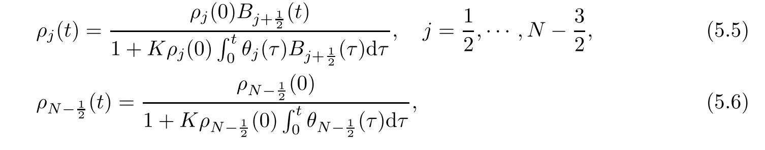
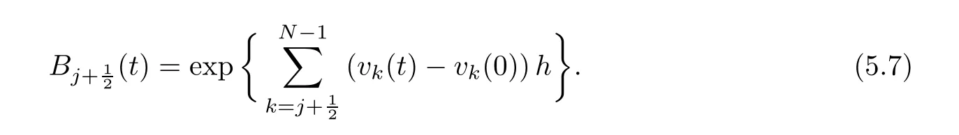
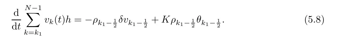
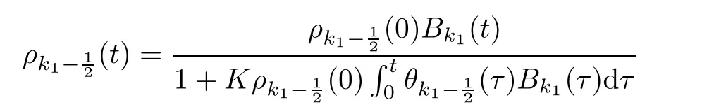
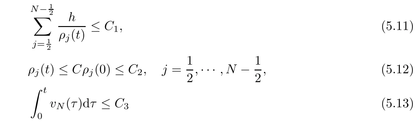
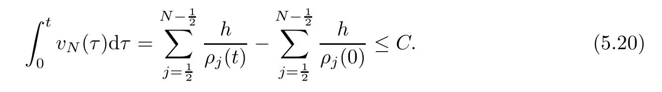
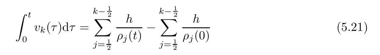
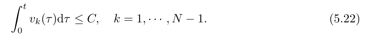
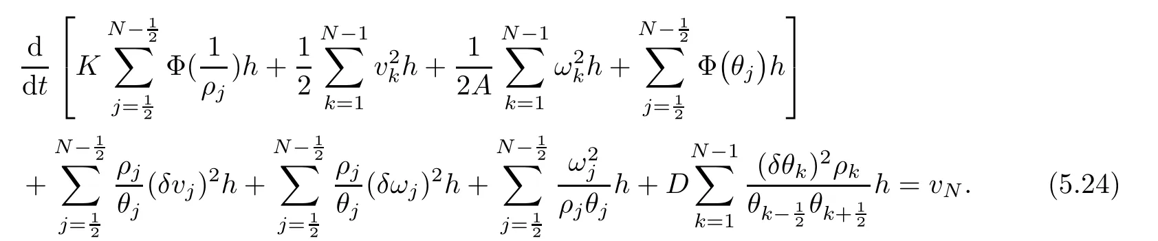
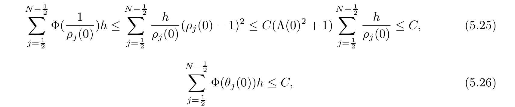
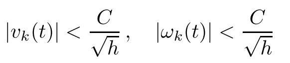
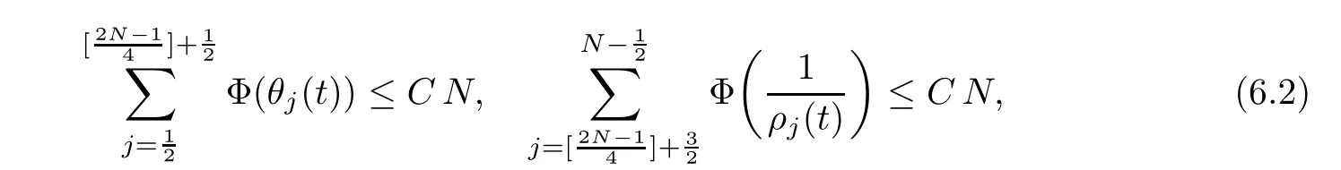
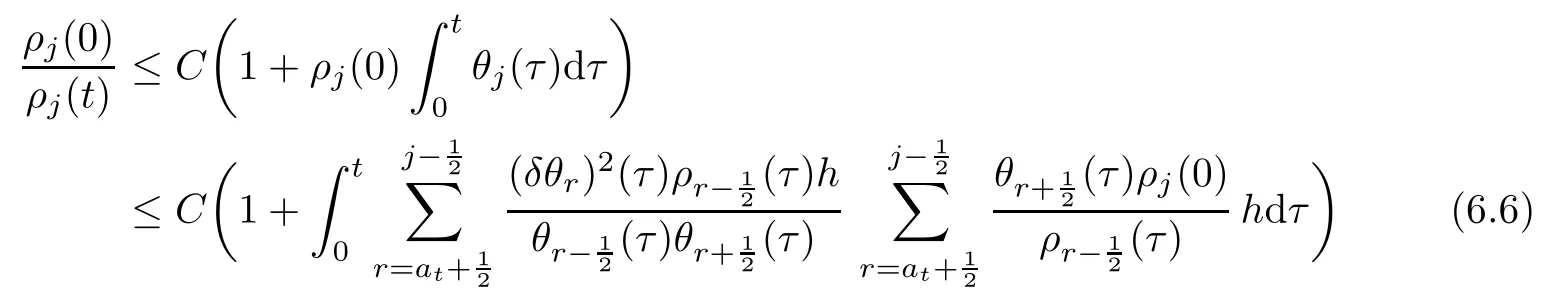
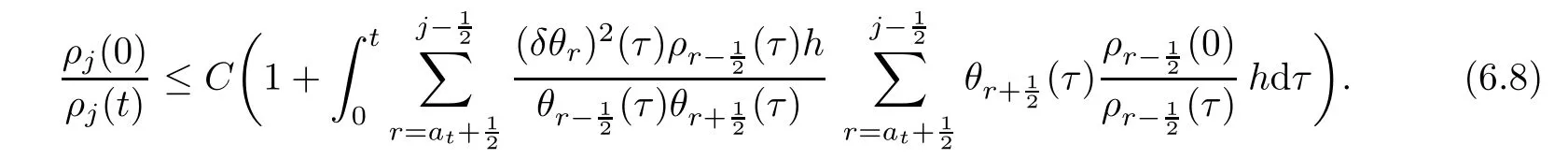
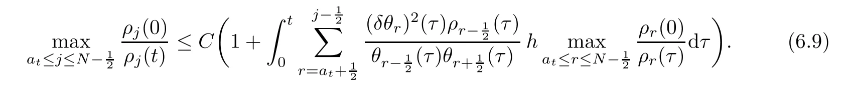
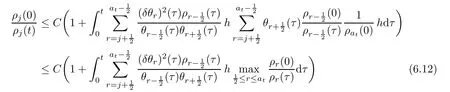
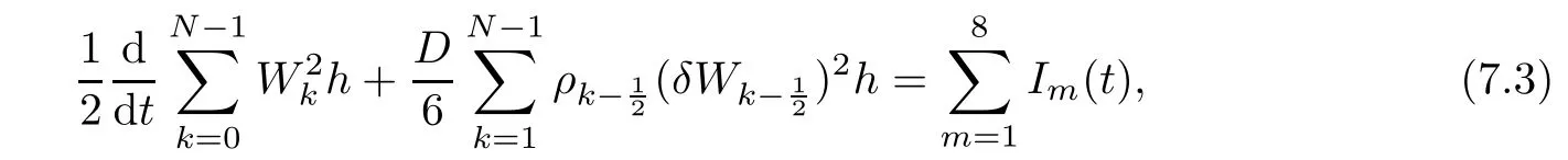
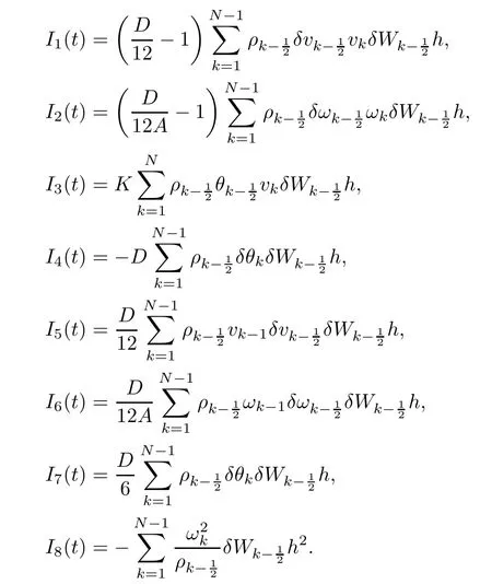
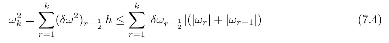
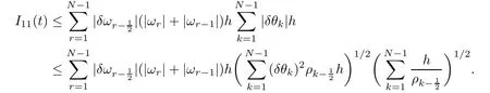
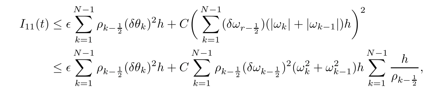
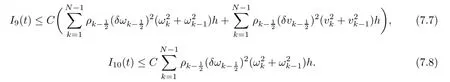
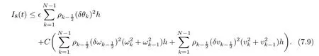
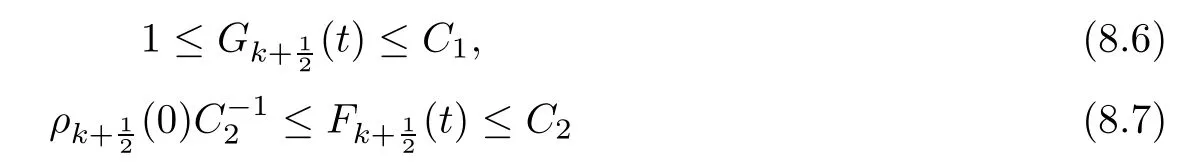
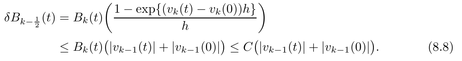
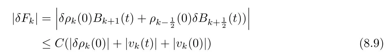
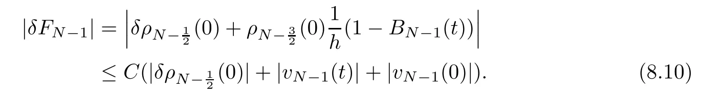
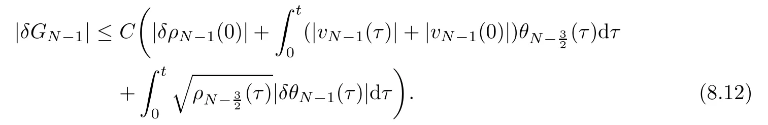
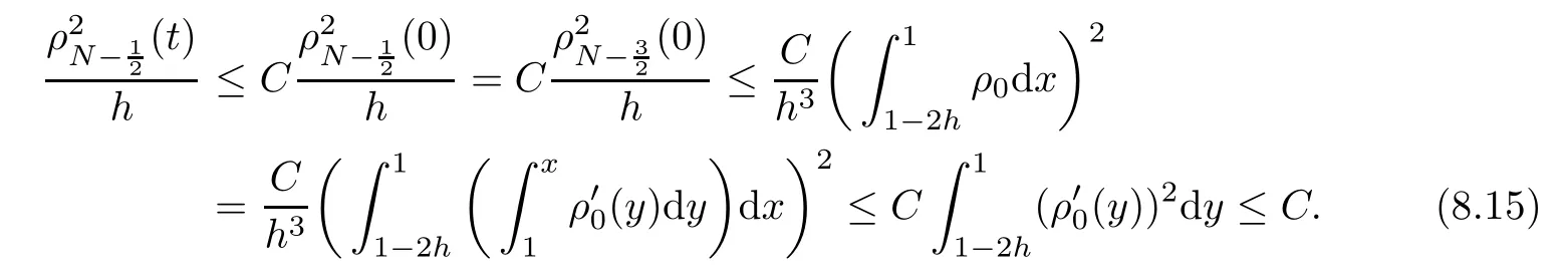
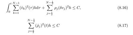
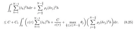
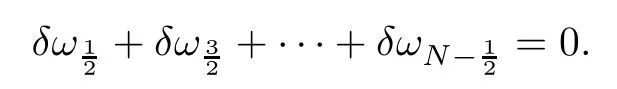
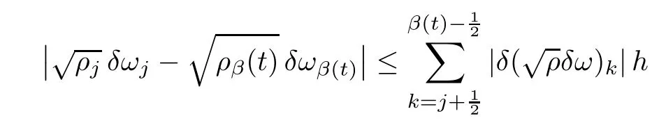
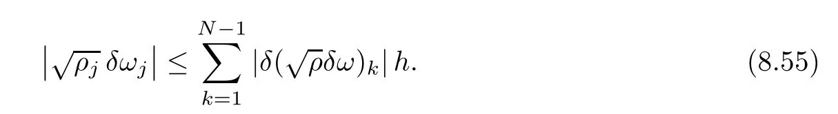
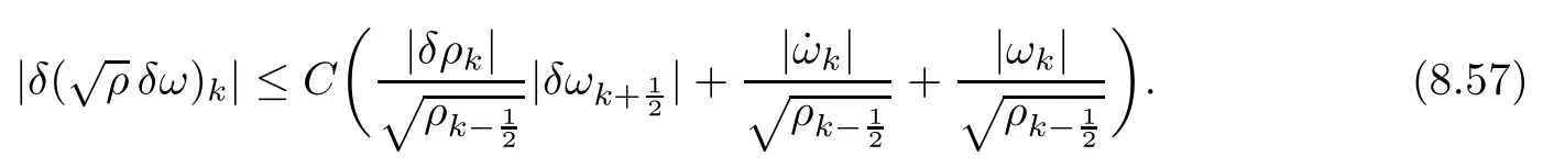
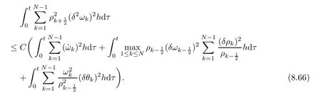
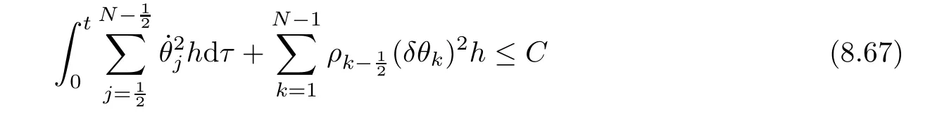
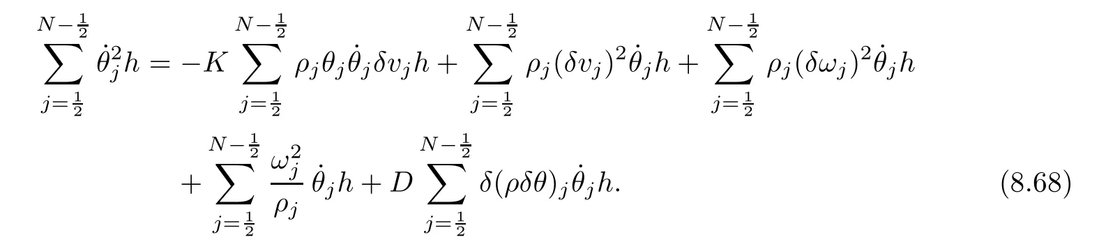
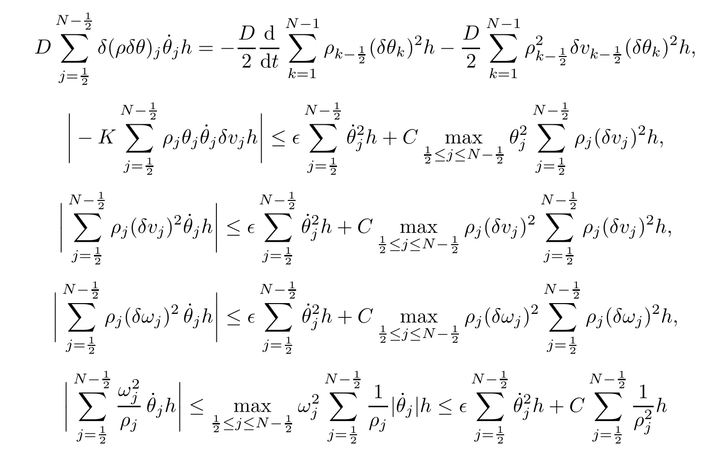
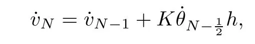
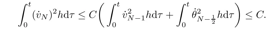
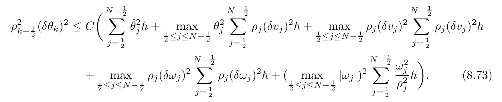
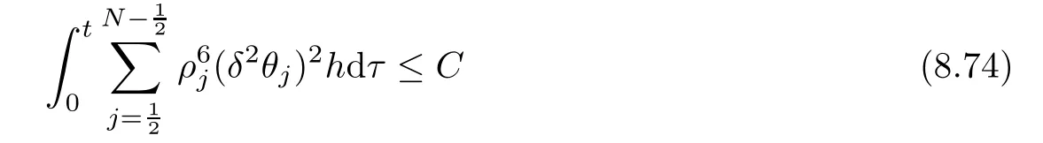
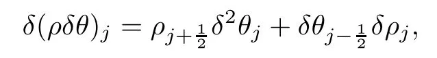
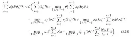
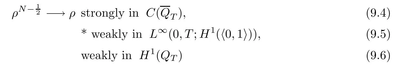
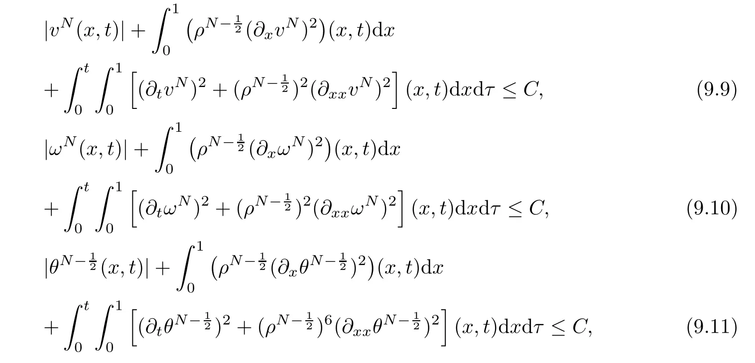
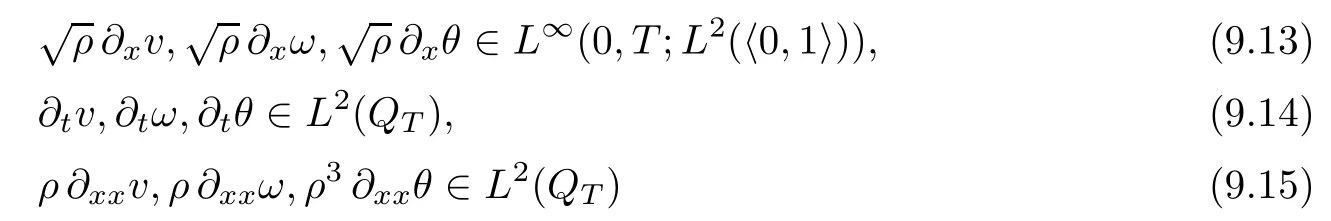
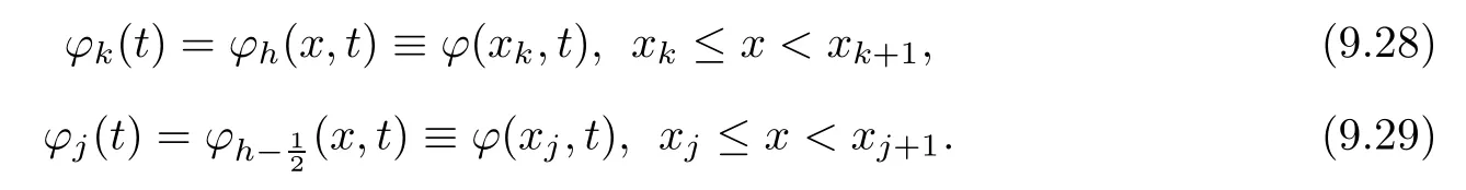
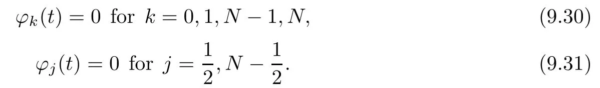
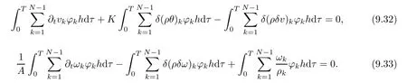
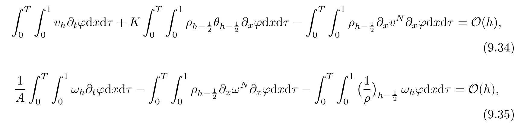
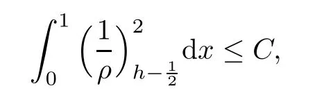
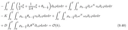
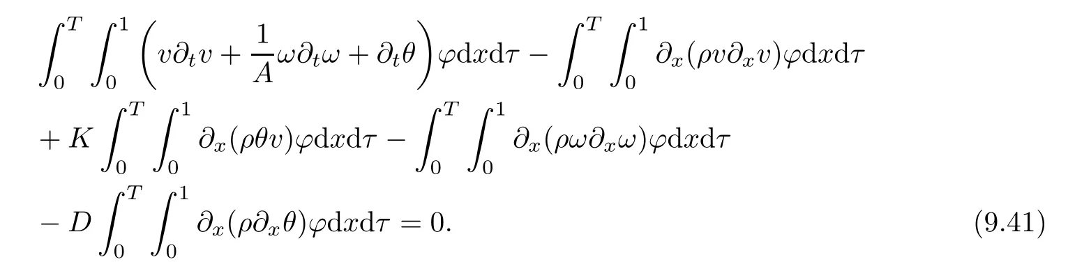
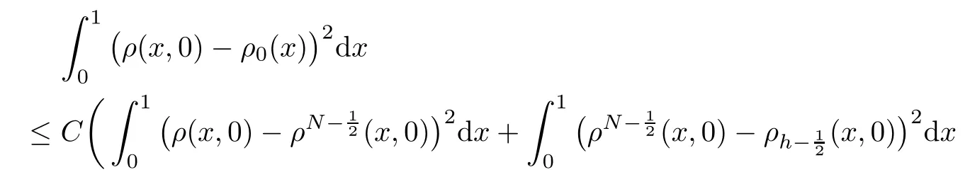
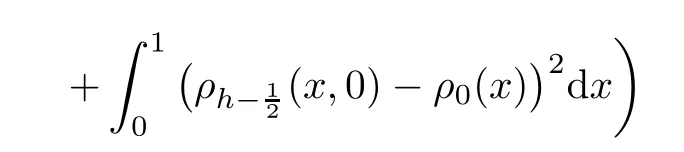
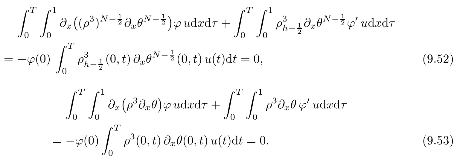
From the basic theory of diferential equations and the local existence theorem,it is known that there exist a smooth solution of the Cauchy problem(3.3)–(3.6),(3.9)–(3.10)with the initial conditions(3.11)–(3.15)on some time interval[0,T0i(see[8,9]),T0 for t∈[0,T0i.Let[0,Tmaxi be the maximal time interval on which the smooth solution satisfying(3.22)and(3.23)exists.Our frst goal is to show that the solution is defned on [0,Ti,i.e.,that Tmax=T.In the similar way as in[4],we will achieve this by showing,for fxed h>0,the boundedness of the mass density,the velocity,the microrotation velocity,the temperature,as well as the lower boundedness of the density and the temperature away from zero(see Section 5).Due to the fact that the estimates we will obtain depend only on T and initial functions,we conclude that the solution(ρj,vk,ωk,θj),j=12,···,N?12,k=0,···,N can be defned on[0,Ti. Now,using the solution of the Cauchy problem(3.3)–(3.6),(3.9)–(3.15)we construct for t≥0 the following approximate functions. For each fxed N,h=1Nx∈[xk,xk+1],k=0,···,N?1,we defne and similarly for x∈[xj,xj+1],j=12,···,N?32,we defne For x∈[0,12N],we take and for x∈[1?12N,1] We also introduce the corresponding step functions: The aim of this paper is to prove the following statements. Theorem 4.1Suppose that the initial data(ρ0,v0,ω0,θ0)satisfy conditions(2.9)–(2.12). Then the initial–boundary value problem(2.1)–(2.7)has a global solution(ρ,v,ω,θ)in the domain QT(for each T∈R+),having the properties There exists a constant C∈R+such that for(x,t)∈QTit holds The proof of Theorem 4.1 is essentially based on a careful examination of a priori estimates and a limit procedure.We frst study,for each N,the approximate problem(3.3)–(3.6),(3.9)–(3.15)and derive the a priori estimates for its solution independent of N(or h)by utilizing a technique of articles[4–6].Using the obtained a priori estimates and results of weak and strong compactness[10,11],we extract the subsequences of approximate solutions,which, when N tends to infnity(or h→0),have the limit in the strong or weak sense on the domain QT=h0,1i×h0,Ti,where T>0 is arbitrary.Finally,we show that this limit is the solution to our problem. Because of the fact that the system(2.1)–(2.4)is considered in[4]using the same method, some of our considerations are similar or identical to those of article[4].In these cases we omit proofs or details of proofs,making reference to correspondent results of article[4].In this article we use some ideas from[12],also.The proof of Theorem 4.1 is a direct consequence of the results that we obtain in the following sections. Throughout this paper,we denote by C>0 or Ci>0(i=1,2,···)generic constants independent of N(i.e.,h),having possibly diferent values at diferent places. In order to construct a global diferential scheme,in this section we frst make some key relations and estimations for(ρj,vk,ωk,θj)(t),j=12,···,N?12,k=0,···,N on the domain [0,Tmaxi,Tmax In the following two lemmas we have the estimations which are formed in the same manner as in[4]. Lemma 5.1(see[11,Lemma 5.4]) There exists C>0 such that for t∈[0,Tmaxi,it holds (C depends only of initial functions ω0). Lemma 5.2There exists C>0 such that for t∈[0,Tmaxi it holds (C depends only of initial functions v0,ω0and θ0). ProofIn the same way as in(see[4],Lemma 5.3)we obtain Using(5.3)from(3.10)we get the estimation for v2N(t)h as follows Lemma 5.3For t∈[0,Tmaxi it holds ProofBy summing(3.4)over k=k1,···,N?1,k1∈{1,···,N?1},we get By inserting(3.3)into(5.8)and integrating over[0,t]it follows where Bk1is defned by(5.7). By multiplying(5.9)by Kθk1?12and integrating over[0,t]again,we obtain From(5.9)and(5.10)follows for each k1∈{1,···,N?1}.Using condition(3.10),in the same way for j=N?12,from (3.4)we get(5.6). ? Lemma 5.4There exist Ci>0,i=1,2,3 such that,for t∈[0,Tmaxi(Tmax hold(C1,C2and C3are dependent of T). ProofNotice that because of(3.19)and(5.2)for the function vk,k=1,···,N,we conclude that there exists C∈R+,C>1,such that for all t∈[0,Tmaxi and j=12,···,N?32.Using(5.14),(5.2)and(3.18)from(5.5)and(5.6) we easily obtain From(5.15)–(5.18),immediately follow(5.11)and(5.12).Now from(3.3)we get the equality Integrating over[0,t]and using(5.11)and(3.18)we easily conclude that Remark 5.1From(3.3)we also get for each k∈{1,···,N?1}and t∈[0,Tmaxi.In the same manner as for vNwe conclude that Lemma 5.5There exists C>0 such that for t∈[0,Tmaxi it holds where Φ(x)=x?1?lnx is a nonnegative convex function. ProofIn the same way as in[4](see Lemma 5.1),from(3.3)–(3.6)we obtain Taking into account estimations(3.16),(2.13)and(5.11)we easily conclude thatuniformly by N.Integrating(5.24)over[0,t],t≤Tmax≤T,and using(3.19),(5.13),(5.25) and(5.26)we get(5.23).Notice that the constant C in(5.23)depends on T. In the similar manner as in[5]or[4]this result verifes the existence of the solution to the Cauchy problem(3.3)–(3.6),(3.9)–(3.15)on the domain[0,Ti,T is arbitrary,i.e.,Tmax=T. Indeed,from(5.23)we get for fxed h>0 that (C depends of T),which implies the global bounds of the functions(ρj,vk,ωk,θj): for each j∈{12,···,N?12}and Hence,we have our construction of the diference scheme(ρj,vk,ωk,θj)(t)defned on[0,Ti for each T>0 and the corresponding approximate solutions on the domain QT. In Lemma 5.4 we show that the functions ρjon[0,Ti,j∈{12,···,N?12}are bounded above.Now we establish the lower bounds for the density and the temperature. Lemma 6.1There exists a constant C1>0 such that for all t∈[0,Ti and j∈{12,···,N?12}it holds ProofFrom(5.23)we have that which implies that there exists,for each t∈[0,Ti,at least one at∈{12,···,[2N?14]+12}andsuch that From(6.3)we conclude that there exists C2∈R+(depends of T)such that Further using the following inequality and estimations(5.14)and(5.12),from(5.5)and(5.6),we get for j∈{12,···,N?12}.First,let be at≤j.Then we have and from(6.6)we conclude that Using(5.2)for the functions θj,from(6.8)it follows By applying Gronwall’s inequality and estimation(5.23),we get Now let be j Using(5.12),(5.2)and(6.11)from(6.6)we obtain and applying Gronwall’s inequality we get again Estimations(6.10)and(6.13)give(6.1). ? Using the upper bound(5.12)for the function ρj(t),j=12,···,N?12,in the same way as in[4]we get the following statement. Lemma 6.2(see[12,Lemma 8.2])There exists C∈R+such that,forand all t∈[0,Ti,it holds First we defne the energy density by for k=0,···,N?1 and t∈[0,Ti.Notice that the function Wkis not the same one as in the article[4].It is easy to see that Wk(t)>0 for each k. We multiply equations(3.4),(3.5),respectively by vkWkh,Wkh and sum up for k=1,···,N?1.We multiply equation(3.6)byand sum up for k=0,···,N?1.Using the equality and following the same procedure as in[4](Section 7),we obtain where In the same way as in[4]we treat I1(t)?I7(t)and obtain inequalities similar to(7.4)–(7.10) from[4].Here we make the estimation for I8(t)only.First,taking into account that and using(7.1)and(5.11),we obtain where For instance,using the Cauchy inequality,from I11(t)we obtain With the help of the Young inequality,we get where ?>0.Because of(5.11)we conclude that In an analogous way as for I11we obtain the inequalities From(7.6)–(7.8)follows For I1(t)?I7(t)we have As in[4],by inserting(7.9)–(7.16)into(7.3),integrating over[0,t]and taking into account (3.21),we conclude(for sufciently small ?>0)that Lemma 7.1There exists C∈R+such that,for t∈[0,Ti,it holds ProofBy using(7.17)and equations(3.4)and(3.5)in the same way as in[4](Lemma 7.1),we obtain(7.18).From(3.10)and(5.2)we conclude that and taking into account(7.18)for the function v4N?1h we get immediately(7.19). ? Lemma 7.2For each t∈[0,Ti,it holds ProofWe use atand b0from Lemma 6.1.First,let be k?12≥at.Then with help of (6.1),(6.7),and inserting inequality(6.5)for θk?12into the right hand side of(7.18),we have By using(3.16),(5.2)and the Young inequality,from(7.21)it follows If we now take that k?12 Using(6.11),(5.2),(5.12)and the Young inequality from(7.23)we conclude that From(7.24)and(7.21)follows By inserting(7.24)into(7.18)and(7.19),we have the inequality Taking into account estimation(5.23)and applying the Gronwall inequality,from(7.25)follows the boundedness of the function for all t∈[0,Ti and(7.20)is obtained. Corollary 7.3Using(3.18)and(7.20),from(5.5)and(5.6)we easily get Now,using(7.20)and(5.12)from(7.24)we easily get for all t∈[0,Ti.With the help of this result,we obtain the following estimations. Lemma 7.4There exists C∈R+such that for all t∈[0,Ti it holds ProofTaking into account(7.27),from(7.18)we get immediately(7.28).Multiplying (3.4)and(3.5),respectively,by v3kh and A?1ρ?1kω3kh,summing over k,using the equality that satisfes(δω3)k?12also and applying the Young inequality with a parameter ?>0,we obtain in the same way as in[4](see(7.16)and(7.17))the inequalities From(7.31)and(7.32)follow(7.29)and(7.30). ? Lemma 7.5There exists C∈R+such that the estimations hold for all t∈[0,Ti. ProofBy multiplying(3.4)by vkh,summing over k=1,···,N?1 and applying the Young inequality with a parameter ?>0,we get By integrating(7.37)over[0,t]and using(3.19),(5.12)and(7.20)(for ? small enough),we obtain(7.33).Taking into account that and applying the Young inequality we get Using(7.29)and(5.11)we easily obtain Analogously,for the function ωkwe get estimations(7.35). Now,let atbe the same as in Lemma 6.1.Then for j≥at(analogously for j From(7.41)follows for j=12,···,N?12.Using(7.28)and(5.11),we get(for small enough ?>0)that We proceed with the further bounds for the variables of the system,needed for proving the main theorem. Lemma 8.1There exists a constant C∈R+such that,for all t∈[0,Ti,it holds ProofIn a similar manner as in[4](Lemma 8.1),from(5.5)and(5.6)we have where for j=12,···,N?32,and (Bj+12is defned by(5.7)).For estimating we need the estimates of the functions(8.3),(8.4),δFkand δGk.Using(3.16),(5.14)and (7.36),we easily conclude that there exist C1,C2∈R+,such that for k=0,···,N?1 and all t∈[0,Ti.Using(5.14)we obtain Now we conclude that for k=1,···,N?2 and Using(5.14),(7.36),(3.16),(8.8)and(5.12),we get for k=1,···,N?2 and for k=N?1 we obtain By applying(8.6)–(8.7)and(8.9)–(8.12),from(8.5)we get Using estimations(3.19),(3.20),(5.2),(7.28)and(7.36),from(8.13)and(8.14),we obtain (8.1). ? For further reasoning we use the property that the initial density vanishes at the free boundary.So we have,with the help of H¨older’s inequality,that Lemma 8.2There exists C∈R+such that hold for all t∈[0,Ti. ProofBy multiplying(3.4)by˙vkh,summing up for k=1,···,N?1 and integrating over[0,t],we obtain Now,we make estimations for the terms on the right–hand side of(8.18).Using(3.16),(3.20), (8.15),(5.2),(5.12),(7.36)and the Young inequality we conclude that Using(3.3),the last integral in(8.18)we can rewrite in the form Notice that,in the similar way as in[5],using σj=ρjδvj?Kρjθj,we have Taking into account(3.4),the Young inequality and that ρj(0)≥ρs(0),for s>j,from(8.23) follows By inserting(8.24)into(8.22)and then(8.19)–(8.22)into(8.18),we conclude that the following inequality holds Using the Gronwall inequality and estimations(7.33)and(7.36)from(8.26)we get With the help of(7.20)we easily conclude that and(8.16)is valid. From(3.3)and(8.16),it immediately follows Note that we did not get the estimation for the function˙v2Nh.It will be obtained later. Lemma 8.3There exists C∈R+such that it holds ProofBy multiplying(3.5)bysumming up for k=1,···,N?1 and integrating over[0,t],we get By using(3.3)and(8.24)with ε(t)=1,for the integrals on the right–hand side of(8.31),we obtain the following inequalities By inserting(8.32)and(8.33)–(8.34)into(8.31),we have and with the help of(7.36)and(8.16),Gronwall’s inequality gives(8.30). ? Corollary 8.4For t∈[0,Ti it holds ProofBy using the H¨older inequality and estimation(8.24),we can easily get Taking into account(5.11),(7.36)and(8.16)we obtain(8.36).From follows(8.37).With the help of(8.16)and(5.11),from the inequalitywe obtain(8.38).Estimation(8.38)we obtain analogously.Taking into account(8.5)–(8.12), we get Because of the embedding,we have ρ0∈C1([0,1])and conclude that With the help of(8.44),(8.38)and(7.36)from(8.43)we obtain and using(5.12),(6.1),(5.11)and(7.28)follows Now we have By using the H¨older inequality from(8.46)we obtain Using(8.30),(7.26),(8.39)and(8.40)from(8.47)follows(8.41). ? By using Corollary 8.4.we obtain the following estimate that will be used in the proceeding. Lemma 8.5There exists C∈R+such that for all t∈[0,Ti it holds ProofBy multiplying(3.5)bysumming over k=1,···,N?1, applying equation(3.4)and integrating over[0,t],we have By using(5.11),(8.30),(8.16),(8.39)–(8.41),(7.26)and the Young inequality,we conclude that By inserting(8.50)–(8.52)into(8.49)(for sufciently ?>0)we obtain(8.48). ? Lemma 8.6For t∈[0,Ti,the estimation is satisfed. ProofFor all t∈[0,Ti,we have It means that,for each t∈[0,Ti,there exists at least one pair of indices α(t),β(t)∈{12,···,N?12}such that Suppose that α(t),β(t)are the smallest indices for which(8.54)is valid.If δωj(t)≥0,then we use δωβ(t)and(for j<β(t))we obtain the inequality and conclude that The same estimate can be obtained for j>β(t).On the other side,if δωj(t)≤0,we use δωα(t)and(for j<α(t)or j>α(t)),we have Using(3.5)we can easily conclude that Inserting(8.57)into(8.56)(or(8.55))and applying the Young inequality we obtain With the help of(8.48),(8.40),(8.30),(5.11)and(5.1)we get(8.53). ? Corollary 8.7It holds ProofUsing(5.12)and(8.53)we have Squaring(8.56)and applying the H¨older inequality and the same estimates as for(8.58)we get (8.60). ? Lemma 8.8There exists C∈R+such that the following inequalities are satisfed. ProofWe rewrite equations(3.4)and(3.5)in the forms from which we easily get Applying(8.16),(5.12),(7.28),(7.36),(8.1),(8.36),(8.40),(8.60)and(8.30)from(8.65)and (8.66)we obtain(8.61)and(8.62). It remains to derive the estimates for the functions θjsimilar as those in Lemmas 8.2–8.8. Lemma 8.9There exists C∈R+such that it holds for all t∈[0,Ti. ProofMultiplying(3.6)byand summing over j=12,···,N?12we obtain Using the following properties and(7.26),(8.16)and(8.30)from(8.68)(for sufciently small ?>0)follows Now we integrate over[0,t],apply the Gronwall inequality and estimations(8.60),(8.36),(8.37) and(7.36)and conclude that(8.67)is valid. Lemma 8.10For j=12,···,N?12and t∈[0,Ti,we have ProofLet atbe the same as in Lemma 6.1.Using(8.67)and(5.11)we easily conclude that Taking into account(8.16),(8.67)and that we get Because of(3.9)we have Inserting δ(ρδθ)jfrom equation(3.6)into(8.72)we get With the help of estimations(8.67),(7.36),(7.33),(8.30),(8.39)and(8.48)from(8.73),we obtain(8.71). Lemma 8.11There exists C∈R+such that it holds for all t∈[0,Ti, ProofBy using the equality ρj?1(t)≥Cρj(t),multiplying(3.6)by ρj,squaring and summing up for j=12,···,N?12,we get With the help of(8.67),(7.36),(5.2),(5.1),(8.16),(8.17),(8.39),(8.40)and(8.71)from(8.75) follows(8.74). In this section we show the compactness of sequences of approximate solutionswhich are defned by(3.24)–(3.31)and their convergence to a solution(ρ,v,ω,θ)of(2.1)–(2.7). First,with the help of estimations(5.12),(8.1)and(8.17)in the same way as in[4],we conclude that there exists C∈R+(independent of N),such that for x∈[0,1]and t∈[0,Ti.Also,using(9.1)we easily get the inequality Estimations(9.1)and(9.2)imply the following statement. Lemma 9.1There exists a function (when N→∞or h→0).There exists a subsequence of(still denotedsuch that The function ρ satisfes the condition where C∈R+. ProofConclusions(9.4)–(9.6)follow immediately from(9.1).From(9.2),we easily get (9.7).By(5.12)and(6.1)the strong convergence(9.4)leads to(9.8). Taking into account estimates(8.38),(8.16),(8.61),(8.70)for the function vN,(8.39), (8.30),(8.62)for the function ωNand estimates(8.69),(8.67)and(8.74)for the function θN?12,we can conclude that there exists C∈R+(independent of N),such that which implies the following statements. Lemma 9.2There exist functions with the properties (when N → ∞ or h→ 0).There exists a subsequence of(still denotedsuch that There exists C∈R+such that ProofConclusions(9.16)–(9.19)follow immediately from inequalities(9.9)–(9.11).Notice that using(9.9),we get the inequality The inequalities of the same form are also valid for the couples of functions ωN,ωhandWith the help of(9.22),we conclude that(9.20)is true.Estimation(9.21)follows from (6.14). Notice that according to(3.11)–(3.13),we have The results that follow in the remaining lemmas are very similar to those of[4]. Lemma 9.3The functions ρ and v defned by Lemmas 9.1 and 9.2 satisfy equation(2.1) a.e.in QT. ProofFirst,we use thatstrongly inand conclude From(9.24)follows For any test function ?∈D(QT)from(9.26)we obtain Convergence(9.25)and its consequence is used for achieving convergence of the second integral in(9.27).Using(9.4),(9.6),(9.17),from(9.27)immediately follows for all ?∈D(QT). Lemma 9.4The functions ρ,v,ω and θ defned by Lemmas 9.1 and 9.2 satisfy equations (2.2),(2.3)and(2.4)a.e.in QT. ProofNow,in the same way as in[4],we choose N=1hlarge enough so that the support of the test function ? is away enough from the boundaries,that is supp??(h,1?h)×(0,t). Defne We can see that Multiply equations(3.4)and(3.5),respectively,by ?kh andsum it up for k=1,···,N?1 and integrate over[0,T]to get Since ?h→?,δ?h→?x?,?t?h→?t? strongly converge as h→0,we can write(9.32)and (9.33)as follows where O(h)→0 as h→0. Now,taking into account that from(7.26)follows we conclude that there exists a subsequencewith the property By using convergences(9.20),(9.7),(9.17)and(9.36)we get that the functions ρ,v and ω satisfy equations(2.2)and(2.3)a.e.in QT.In the same way as in[4],multiplying(3.4)–(3.6), where O(h)→0 as h→0.After summing the above equations we get Because of(9.7),(9.16)and(9.17),from(9.40),for h→0,follows Now,already proven equations(2.2)and(2.3)we multiply,respectively,by v? and A?1ρ?1ω?, integrate over QTand add up to(9.41).So we get that(2.4)is satisfed. ? Lemma 9.5The functions ρ,v,ω and θ satisfy the following conditions for x∈h0,1i and t∈h0,Ti(ρ0,v0,ω0and θ0are introduced by(2.12)). ProofFrom the following inequality with the convergences(9.4),(9.2)and(9.23),we can easily conclude that ρ(x,0)=ρ0(x), x∈h0,1i.Analogously we get that v(x,0)=v0(x),ω(x,0)=ω0(x),θ(x,0)=θ0(x),x∈h0,1i. Notice that from(8.48),(8.36),(8.71),(5.11)and(7.26)we have and we conclude that weakly in L2(QT). Therefore we can apply Green’s formula as follows.First,we take ?∈C∞([0,1])with the property ?(0)6=0 and that is equal to zero at some neighborhood of point 1.Let be u∈L2(h0,Ti).It holds For the function v we have also Taking into account that vN(0,t)=0 and comparing(9.49)and(9.50),when N → ∞,we obtain In the same way we get ω(0,t)=0. Taking into account that?xθN?12(0,t)=δθ0(t)=0 and using the Green’s formula we have Applying(9.48),(9.7),(9.17)and comparing(9.52)and(9.53),when N→∞,we get Taking ?∈C∞([0,1])with the property ?(1)6=0 and that is equal to zero at some neighborhood of point 0,we conclude as in(9.49)and(9.50),that and,as in(9.52)and(9.53) Applying the property and that weakly in L2(QT),we have Green’s formula in the following forms for u∈L2(h0,Ti).With the help of strong convergence(9.7)and(9.20)from(9.59)and(9.60) we obtain Corollary 9.6From(9.47)and(9.48)we know that The results from the lemmas in Section 9 give statements of Theorem 4.1. In this paper the fnite diference scheme for the nonstationary 1D fow of the compressible viscous and heat-conducting micropolar fuid,which is in the thermodynamical sense perfect and polytropic,with the homogeneous boundary conditions for velocity,microrotation and heat fux,is defned and analyzed.The sequence of the approximate solution is constructed as a solution of the fnite diference approximate equations system,which is derived by using the appropriate fnite diference spatial discretization.The properties of these approximate solutions are analyzed and their convergence to the strong solution of our problem globally in time is proved.In this way the global existence of the solution is verifed.The numerical properties of the proposed scheme are presented on the chosen test example. [1]Mujakovi′c N.One-dimensional fow of a compressible viscous micropolar fuid:a local existence theorem. Glasnik Matematiˇcki,1998,33(53):71–91 [2]Mujakovi′c N.Non-homogeneous boundary value problem for one-dimensional compressible viscous micropolar fuid model:a local existence theorem.Annali Dell’Universita’Di Ferrara,2007,53(2):361–379 [3]Mujakovi′c N.The existence of a global solution for one dimensional compressible viscous micropolar fuid with non-homogeneous boundary conditions for temperature.Nonlinear Anal-Real,2014,19:19–30 [4]Mujakovi′c N,ˇCrnjari′c-ˇZic N.Convergent fnite diference scheme for 1d fow of compressible micropolar fuid.Int J Num Anal Model,2015,12:94–124 [5]Chen G Q,Kratka M.Global solutions to the Navier-Stokes equations for compressible heat-conducting fow with symmetry and free boundary.Comm Partial DifEqs,2002,27:907–943 [6]Chen G Q,HofD,Trivisa K.Global solutions of the compressible Navier-Stokes equations with large discontinuous initial data.Comm Partial DifEqs,2000,25:2233–2257 [7]Lukaszewicz G.Micropolar Fluids.Boston:Birkh¨auser,1999 [8]Arnold V I.Ordinary Diferential Equations.Cambridge:MIT Press,1978 [9]Petrowski I G.Vorlesungen¨uber die Theorie der gew¨ohnlichen Diferentialgleichungen.Leipzig:Teubner, 1954 [10]Doutray R,Lions J I.Mathematical Analysis and Numerical Methods for Science and Technology,Vol 2. Berlin:Springer-Verlag,1988 [11]Doutray R,Lions J I.Mathematical Analysis and Numerical Methods for Science and Technology,Vol 5. Berlin:Springer-Verlag,1992 [12]Antonsev S V,Kazhinkhov A V,Monakhov V N.Boundary Value Problems in Mechanics of Nonhomogeneous Fluids.Studies in Mathematics and its Applications,Vol 22.Amsterdam:North–Holland Publ Co, 1990 ?Received March 10,2015;revised April 29,2016.This work was supported by Scientifc Research of the University of Rijeka(13.14.1.3.03).


4 The Main Result

5 Basic Relations and Estimates,Global Construction of the Diference Scheme


6 Lower Bounds for the Density and the Temperature


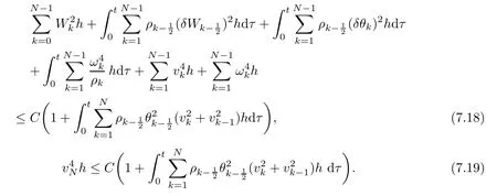
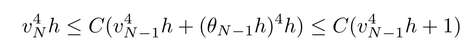
7 Boundedness of the Energy Density and Its Consequences


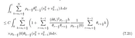
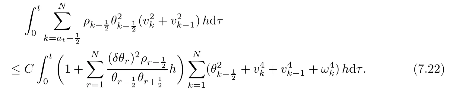


8 Further Bounds for the Density,Velocity,Microrotation Velocity and Temperature


9 Convergence of Approximate Solutions to a Solution of(2.1)–(2.7)


10 Conclusion
 Acta Mathematica Scientia(English Series)2016年6期