Output feedback robust model predictive control with unmeasurable model parameters and bounded disturbance☆

Baocang Ding*,Hong guang Pan

Ministry of Education Key Lab For Intelligent Networks and Network Security,Department of Automation,School of Electronic and Information Engineering,Xi'an Jiaotong University,Xi'an710049,China

1.Introduction

Consider a process system model

whereare the input,state,output and bounded disturbance,respectively.This model has been widely studied(see e.g.[1]).For the time-varying[A|B|C|D|E](k)lying in a polytope,two kinds of uncertainties have been considered.One,which is referred to as the quasi-uncertain linear parameter varying(LPV),assumes that[A|B|C|D|E](k)are exactly known at the current time k albeit unknown in the future.The other,which is referred to as the uncertain LPV,assumes that[A|B|C|D|E](k)are unknown for all k.

For the case when w(k)is persistent and unknown,we have published several works for output feedback robust MPC(OFRMPC)(see Table1).In these previous works,we have developed the following effective technical tools:

(1)norm-bounding technique for handling physical constraints.Some scalars(norm bounds)are utilized to counteract the effect of w(k).These scalars are off-line optimized,so that the conservatism is reduced for constraint handling.

(2)the notion of quadratic boundedness(QB)and dynamic output feedback law.QB describes quadratic convergence outside of an ellipsoid and invariance inside of this ellipsoid,which is concise for specifying stability property.The dynamic output feedback has four control parametric matrices,which can admit desirable solutions for the uncertain LPV models(the computational burden can be reduced by pre-fixing two control parametric matrices),and parameter-dependent efficient solutions for the quasi-uncertain LPV models.

(3)the ellipsoidal and polyhedral state estimation error bounds(EEBs).The ellipsoidal and polyhedral sets are widely utilized in the control theory.We utilize both kinds of sets which have complementary advantages.

(4)the auxiliary optimization problem for determining the time for performing the main optimization,which also reduces the on-line computational burden.An inappropriate refreshment of the main optimization problem may not yield the feasible solutions,and it is unnecessary that receding-horizon optimization always improves the control performance.

(5)the ellipsoid refreshment formula for guaranteeing the recursive feasibility.By a simple refreshment of the ellipsoidal EEB,the recursive feasibility can be guaranteed.

As shown in Table 1,not every previous work utilizes all the above five tools.Previously,the above tools were not fully utilized due totechnical difficulties.In our recent works[16,17],in the context of polyhedral disturbance bound and uncertain LPV model,the above techniques(1),(2)and(3)have been merged.In this paper,we summarize the results in[16]and[17],and give a set of algorithms for OFRMPC;this is mainly related to[4],[6],and[8],for which more comparisons are shown in the following.

Table 1 The differences between this paper and the existing works

The work[6] firstly applies the following dynamic output feedback controller for MPC of the uncertain LPV system:

whereis the controller state;{Ac,Lc}(k)are controller gain matrices;{Fx,Fy}(k)are feedback gain matrices.Indeed,before[6],the works[5,8]apply the same feedback controller,albeit Fy=0 and originally discussing the estimator-based output feedback.In the context of OFRMPC,one of the major difficulties is refreshing EEBs.The works[5,6,8]add the estimation error constraint(EEC)in the main optimization problem which imposes that the estimation error has to evolve within the polyhedral EEBs.Adding EEC simplifies OFRMPC since it is no longer required to refresh EEB.However,EEC has its adverse effects,such as degrading the control performance and shrinking the region of attraction.In[2]and[14],EEC is removed,and the auxiliary optimization problems are utilized to refresh EEBs.By applying the polyhedral EEBs(see[2,5,6,8,14]),the recursive feasibility of the main optimization problem is not guaranteed.By applying the ellipsoidal EEB(see[3,4,7,15]),it begins to guarantee the recursive feasibility.

Some previous works are not for uncertain LPV models,e.g.,[2]and[3]study the quasi-uncertain LPV models and[5,7]consider Hammerstein–Wiener model.The works[5]and[7]are based on those for uncertain LPV models,i.e.,[8]and[4],respectively.By removing EEC and optimizing more controller parameters,[4]improves[8],so[7]improves[5].In the present paper,we study the uncertain LPV model which is more general and sophisticated,so the results can be extended to the quasi-uncertain LPV and Hammerstein–Wiener models.

There are several more differences among[4],[6],and[8].The work[8]applies the dilation technique to handle the linear matrix inequalities(LMIs),while[4]and[6]abandon this technique.The work[8]uses the norm-bounding technique to handle the invariance conditions,while[4]and[6]utilize the notion of QB.The works[6,8]pre-specify a part of control law parameters for simplification,while[4]optimizes all the controller law parameters.The work[8]assumes polyhedral bound of w(k)and utilizes the norm-bounding technique to simplify the LMIs,while[4]and[6]assume ellipsoidal bound of w(k)but give up the norm-bounding technique.

By fusing the merits and erasing the differences,the present paper has three notable contributions:(1)the constraint handling results are improved by the norm-bounding technique;(2)some previous techniques in[4],[6]and[8]are shown to be special cases;(3)it paves the way,so it can be the new starting point,for the future researches.

Notations:For a vector x and positive-definite matrix,and x(i|k)is the value of x(k+i)predicting at time k.I is the identity matrix with appropriate dimension.Co｛S｝denotes a convex hull,i.e.,any element belongs to Co｛S｝ is a combination of elements in the polytope S,with the scalar combing coefficients being nonnegative and summing as 1.The symbol?induces a symmetric structure in a square matrix.For the MPC decision variables,the time indices are often omitted for simplicity.

2.Problem Statement

Based on the predictions made by Eqs.(1),(2),the augmented prediction model at time k is

2.1.System assumptions and notion of quadratic boundedness

The following is a general assumption of this paper.

The following assumption(1)is equivalent to,while(2)is a special case of,Assumption 1:

The results in this paper are based on Assumption 1,but are more tightly suitable for the above Assumptions A1–A2.

The notion of QB,originally inherited from[9]and[10],can be utilized on Eq.(3).

Definition 1.The system(3)is quadratically bounded with a common Lyapunov matrixif,for all allowable λj(k+i)and w(k+i),i≥ 0,

2.2.Optimization problem

In the dynamic OFRMPC,let us solve,at each time k,

If Eq.(12)holds,then Eq.(13)guarantees Eq.(8).Applying the Schur complement,it is shown that Eqs.(12),(13)are equivalent to Eqs.(14),(15).

3.Synthesis Approaches of Dynamic OFRMPC

We firstly propose a general approach to the dynamic OFRMPC,incorporating the relaxation scalars,in Section 3.1,and then simplify it in Section 3.2 by pre- fixing a part of the control parameters.In Section 3.3,we off-line optimize the relaxation scalars finishing the norm-bounding technique.

3.1.A general synthesis approach of dynamic OFRMPC

A specific synthesis approach of OFRMPC is dependent on how to handle Eqs.(7),(9)and(10).

Applying Eq.(18)and the following proposition,the physical constraints are handled.

Applying the Schur complement,it is shown that Eq.(24)is equivalent to Eq.(20).

In Lemma 4,η1s(s=1,…,nu),η3s,η4s(s=1,2,…,q)are the relaxation scalars.Lemma 4 keeps unchanged if we replace w(k)by w(k)σ(k)where σ(k)∈ Co{?1,1}is unknown and persistent.

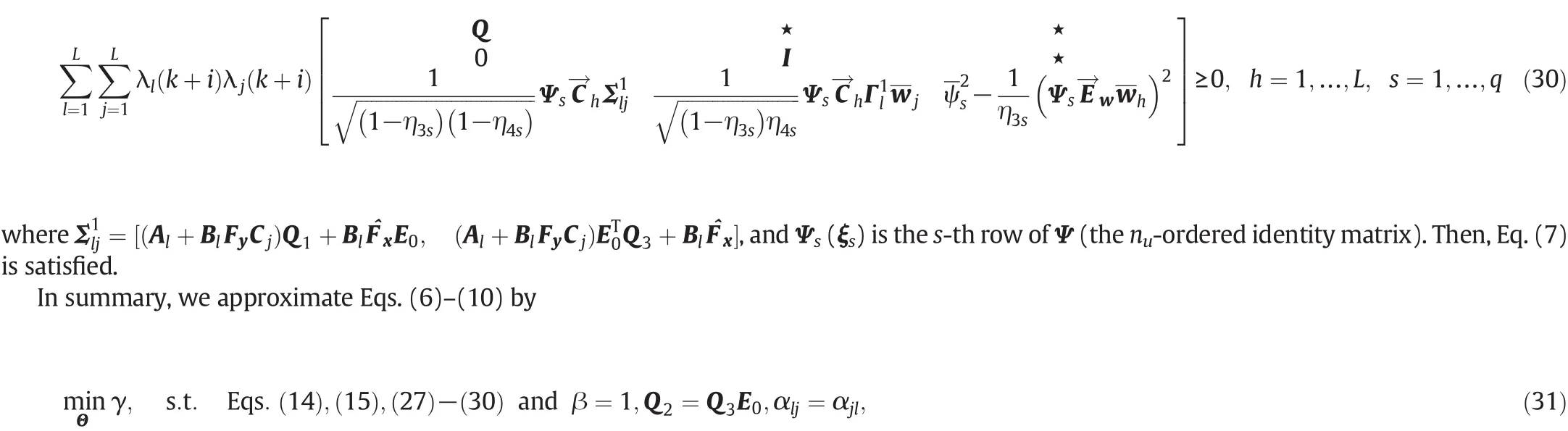
Summarizing Lemmas 2,3 and 4,we approximate Eqs.(6)–(10)by

at time k=0,and Assumption2 holds,and Me(k)is refreshed according to

3.2.A simplified synthesis approach of dynamic OFRMPC

By the simplified approach,we refer to the case when Lcand Fyare pre-specified.The pre-specification ofis shown in Algorithm 1 in the sequel.Take the transformationsTakeApplying a congruence transformation,via diag{Q,I},it is shown that Eqs.(16),(17)hold if

whereA comparison of the problems(25)and(31)are shown in Table 2.For Eq.(25),there are two sources of heavy computational burden(see[4,14]):(1)cone complementarity approach for achieving M=Q?1,which often increases the computation burden for dozens of times;(2)iterative approach for minimizing γ,which often increases the computation burden for a few to hundreds of times.Therefore,Eq.(25)involves dozens to thousands of times larger computational burden than Eq.(31).For practical applications,it is more suitable to apply Eq.(31)than to apply Eq.(25).

Table 2 A comparison of Eqs.(25)and(31)

The closed-loop stability by applying Eq.(31)is similar to that by Eq.(25).

Corollary 1.For the system(1),the dynamic OFRMPC is adopted withobtained via solving Eq.(31).If Eq.(31)is feasible at time k=0,and Assumption 2 holds,and Me(k)is refreshed according to

at each time k＞0,then ｛～x，u｝ will converge to a neighborhood of{0,0},and Eqs.(4),(5)are satisfied for all k≥0.

3.3.Pre-specifying relaxation scalars by norm-bounding technique

In both Eqs.(25)and(31),line searching ηrss considerably increases the computational burden.In[8],the similar scalars are eliminated(from on-line optimization)by applying the norm-bounding technique.In the following,we pre-specify ηrss by the extended norm-bounding technique.

Lemma 6.In the problem(31),the conditions(29),(30)hold if

Proof.By takingas in Eq.(37),and congruence transformation on Eq.(29)via

4.Applying to Different System Assumptions

Firstly,Eqs.(25)and(31)are applied to a set of special system assumptions.Then,taking[8]as an example,it is shown that some previous approaches are special cases.

4.1.Applying to a set of special system assumptions

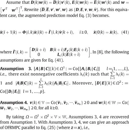
whereThe closed-loop stability holds the same as Eq.(25).

With Assumptions 3,4,we can also give a simplified approach of OFRMPC parallel to Eq.(31)(where z=x),i.e.,

4.2.Reformulation of a previous approach as a special case

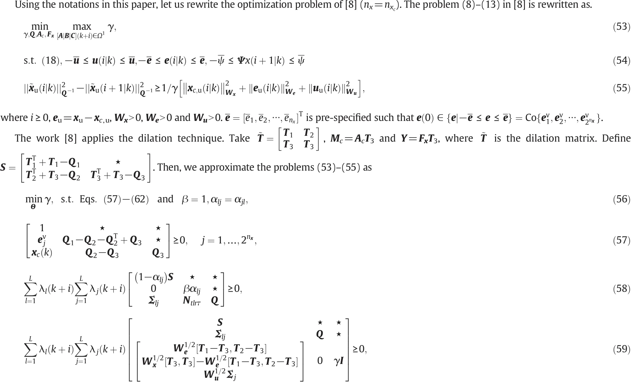
Remark 3.Introducing～T changes the numerical solutions,and can be influential for the receding-horizon implementation.However,～T has an adverse effect on feasibility.The congruence transformation does not affect the feasibility.If Eq.(56)is infeasible,but becomes feasible when～TT+～T?Q is replaced by～TTQ?1～T,then it is the special structure of～T which leads to infeasibility;one cannot take～T=Q(see[18])to deny this fact,since Eq.(56)does not take Q2=Q3.Only when Q2=Q3is specified,the above special structure of～T will not affect the feasibility.

Proposition 2.Problem(56)is less conservative than Eq.(22)in[8](which approximates the problems(8)–(13)in[8]),i.e.,the latter is a special case of the former.

Proof.Refer to Proposition 1 in[17].

We cannot show that Eq.(56)(or Eq.(22)in[8])is a special case of Eq.(46).Anyway,Eq.(56)(and Eq.(22)in[8])utilizes the full Q and～T.Besides the full Q and～T,Eq.(46)is better than Eq.(56).As compared with Eq.(46),there are two weaknesses in Eq.(56):(1)the loss of recursive feasibility;(2)the intrusion of conservatism(both in feasibility and optimality)by imposing EEC.In order to guarantee recursive feasibility,Eq.(56)can be modified with Q2=Q3E0and Lemma 2;in such a case,by further taking～T=Q we can say that Eq.(46)includes the modified optimization problem as a special case.

Indeed,it is easier to show that the techniques in this paper include the counterparts in[4]and[6]as special cases.

Remark 4.The approaches in this paper are computationally formidable for moderate or large dimensional systems.One can use the off line MPC,which off-line optimizes a series of{Ac,Lc,Fx,Fy,Q}corresponding to a series of off-line selected{Me,xc}(stored in the look-up table),and on-line(at each time k≥0),chooses a set of{Ac,Lc,Fx,Fy}(k)(among the look-up table)according to the real-time{xc,Me,ρ}(k).This is a usual procedure of gain-scheduling control,which is not detailed here.

5.Illustrative Example

We obtain the model parameters by handling the model of a continuous stirred tank reactor (CSTR) for an exothermic, irreversible reaction.For the physical meaning of CSTR model, refer to [13]. The model parameters corresponding to Eq Eq.(1)are:L=4,

At k=0,Eq.(56)is infeasible for any xc(0)andwhich means that the procedure in[8]cannot be applied.In the sequel we simulate the following three methods:

Mthd 1:applying Eq.(25),where ηrss are pre-specified as

Mthd 2:similar to Mthd1,but ηrss are optimized according to Algorithm 1;

Mthd 3:applying Eq.(31),where ηrss are optimized according to Algorithm 1.

In Mthd1–Mthd3,forEq.(25)and Algorithm1,choose{N0,d,d0,κ}={200,0,0,0.98}(see[4,14]:N0is the maximum allowable amount of iterations in the cone complementarity approach;d and d0are the complexity index and the maximum complexity index for handling the DbCCs,respectively;κ is the accuracy for minimizing γ).Mthd1 and Mthd2 differ in whether or not ηrss are optimized.Mthd2 and Mthd3 differ in whether or not{Fy,Lc}are on-line optimized.

Fig.1.The regions of attraction,set(1).

Here,the region of attraction,say Xc,is the region of xc(0)such that,whenever xc（0）∈Xc,the optimization problem is feasible.Some further results are shown in Figs.3–6.The evolution of γ,as in Figs.3,4,represents the control performance since we consider the min–max optimization in this paper.By observing Figs.1–4,we obtain the following conclusions:

Fig.2.The regions of attraction,set(2)

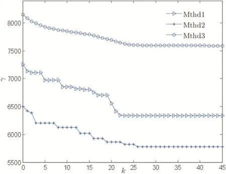
Fig.3.The evolution of γ,set(1).

Fig.4.The evolution of γ,set(2).

Fig.5.The state trajectory of the closed-loop system,set(2).

Fig.6.The control input signal,set(2).

(1)By comparing Mthd1 and Mthd2,it is shown that optimizing ηrss can enlarge the region of attraction and improve the control performance.

(2)By comparing Mthd2 and Mthd3,it is shown that optimizing{Fy,Lc}can enlarge the region of attraction and improve the control performance.

(3)In Fig.1,the region of attraction of Mthd3 even encloses that of Mthd1,while in Fig.2 this phenomenon does not appear.The pre-specified Lcand Fygreatly influence the region of attraction and the control performance.

For Mthd1–Mthd2,since κ=0.98,i.e.,2 percent minimization error can be observed, the comparisons should be made by allowing this inaccuracy(e.g.,in Figs.3–4,the curves for Mthd1–Mthd2 decrease very slowly or very sharply at some sampling instants).While on-line optimizing{Fy,Lc}is advantageous for control performance and region of attraction,it is disadvantageous for computation.The total amounts of computational time for k≤50(average of sets(1)and(2))by applying Mthd1–Mthd3 are 0.25 h,0.20 h and 135 s respectively.For the state trajectories and control input signals,we only give those for set II for brevity;see Figs.5,6,which verify the closed-loop stability and constraints satisfaction.In summary,the simulation example verifies the basic theoretical results.

6.Conclusions

This paper has presented the synthesis approaches of dynamic OFRMPC which include the previous methods in[4],[6],and[8]as special cases.The techniques for quadratic boundedness,dynamic output feedback,norm-bounding,and recursive feasibility,which were invented in separate works previously,are fused in this paper.It is shown that the fused procedure can improve the control performance and enlarge the region of attraction.We believe that this is useful,and can be a new starting point,for further researches.Based on this paper,a number of issues,such as the refreshment of EEB,the reduction of computational burden,will be studied in the future.

[1]D.F.He,H.Huang,Q.X.Chen,Quasi-min-max MPC for constrained nonlinear systems with guaranteed input-to-state stability,J.Frankl.Inst.351(2014)3405–3423.

[2]B.Ding,Constrained robust model predictive control via parameter-dependent dynamic output feedback,Automatica 46(2010)1517–1523.

[3]B.Ding,Dynamic output feedback predictive control for nonlinear systems represented by a Takagi–Sugeno model,IEEE Trans.Fuzzy Syst.19(2011)831–843.

[4]B.Ding,Dynamic output feedback MPC for LPV systems via near-optimal solutions,Proceedings of the 30th Chinese Control Conference,Yantai,China 2011,pp.3340–3345.

[5]B.Ding,B.Huang,Output feedback model predictive control for nonlinear systems represented by Hammerstein–Wiener model,IET Control Theory Appl.1(2007)1302–1310.

[6]B.Ding,B.Huang,F.Xu,Dynamic output feedback robust model predictive control,Int.J.Syst.Sci.42(2011)1669–1682.

[7]B.Ding,X.Ping,Dynamic output feedback model predictive control for nonlinear systems represented by Hammerstein–Wiener model,J.Process Control 22(2012)1773–1784.

[8]B.Ding,Y.Xi,M.T.Cychowski,T.O'Mahony,A synthesis approach for output feedback robust constrained model predictive control,Automatica 44(2008)258–264.

[9]A.Alessandri,M.Baglietto,G.Battistelli,On estimation error bounds for receding-horizon filters using quadratic boundedness,IEEE Trans.Autom.Control 49(2004)1350–1355.

[10]A.Alessandri,Design of state estimators for uncertain linear systems using quadratic boundedness,Automatica 42(2006)497–502.

[11]A.Sala,C.Arino,Asymptotically necessary and sufficient conditions for stability and performance in fuzzy control:Application of Polya's theorem,Fuzzy Sets Syst.158(2007)2671–2686.

[12]V.F. Montagner, R.C.L.F. Oliveira, P.L.D. Peres, Necessary and sufficient LMI conditions to compute quadratically stabilizing state feedback controllers for Takagi–Sugeno systems,Proceedings of the American Control Conference, NY, USA 2007, pp. 4059–4064.

[13]Z.Wan,M.V.Kothare,Efficient scheduled stabilizing output feedback model predictive control for constrained nonlinear systems,IEEE Trans.Autom.Control 49(2004)1172–1177.

[14]B.Ding,C.Gao,X.Ping,Dynamic output feedback robust MPC using general polyhedral state bounds for the polytopic uncertain system with bounded disturbance,Asian J.Control 18(2015)699–708.

[15]B.Ding,X.Ping,H.Pan,On dynamic output feedback robust MPC for constrained quasi-LPV systems,Int.J.Control 86(2013)2215–2227.

[16]B. Ding, Y. Xi, H. Pan, Synthesis approaches of dynamic output feedback robust MPC for LPV system with unmeasurable polytopic model parametric uncertainty—Part II.Polytopic disturbance, Proceedings of the 27th Chinese Control and Decision Conference,Qingdao, China 2015, pp. 95–100.

[17]B.Ding,Y.Xi,Synthesis approaches of dynamic output feedback robust MPC for LPV system with unmeasurable polytopic model parametric uncertainty—Part III.Reformulation of a previous approach,Proceedings of 5th Annual IEEE International Conference on CYBER Technology in Automation,Control and Intelligent Systems,Shenyang,China 2015,pp.246–251.

[18]M.C.de Oliveira,J.Bernussou,J.C.Geromel,A new discrete-time robust stability condition,Syst.Control Lett.37(1999)261–265.