GENERAL DECAY OF SOLUTIONS FOR A VISCOELASTIC EQUATION WITH BALAKRISHNAN-TAYLOR DAMPING AND NONLINEAR BOUNDARY DAMPING-SOURCE INTERACTIONS?
2015-11-21 07:11:45ShunTangWU吳舜堂
Shun-Tang WU(吳舜堂)
General Education Center,National Taipei University of Technology,Taipei 106,China
GENERAL DECAY OF SOLUTIONS FOR A VISCOELASTIC EQUATION WITH BALAKRISHNAN-TAYLOR DAMPING AND NONLINEAR BOUNDARY DAMPING-SOURCE INTERACTIONS?
Shun-Tang WU(吳舜堂)
General Education Center,National Taipei University of Technology,Taipei 106,China
E-mail:stwu@ntut.edu.tw
A viscoelastic equation with Balakrishnan-Taylor damping and nonlinear boundary/interior sources is considered in a bounded domain.Under appropriate assumptions imposed on the source and the damping,we establish uniform decay rate of the solution energy in terms of the behavior of the nonlinear feedback and the relaxation function,without setting any restrictive growth assumptions on the damping at the origin and weakening the usual assumptions on the relaxation function.
Balakrishnan-Taylor damping;global existence;general decay;relaxation function;viscoelastic equation
2010 MR Subject Classification 35L70;35L20;58G16
1 Introduction
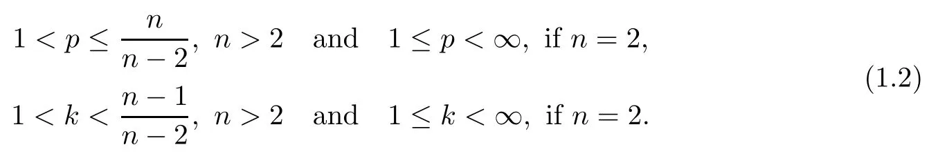
In this paper,we study the following viscoelastic problem with Balakrishnan-Taylor damping and nonlinear boundary/interior sources:
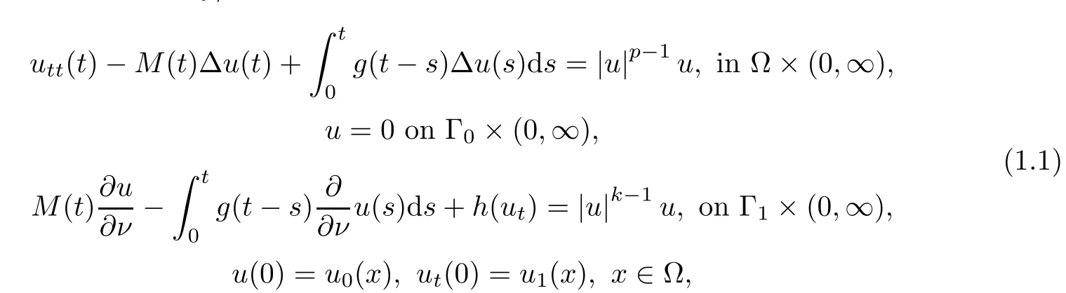
The equations in(1.1)with M≡1 form a class of nonlinear viscoelastic equations used to investigate the motion of viscoelastic materials.As these materials have a wide application in the natural sciences,their dynamics are interesting and of great importance.Hence,questions related to the behavior of the solutions for the PDE system attracted considerable attention in recent years.For example,Cavalcanti et al.[7]considered the following problem:
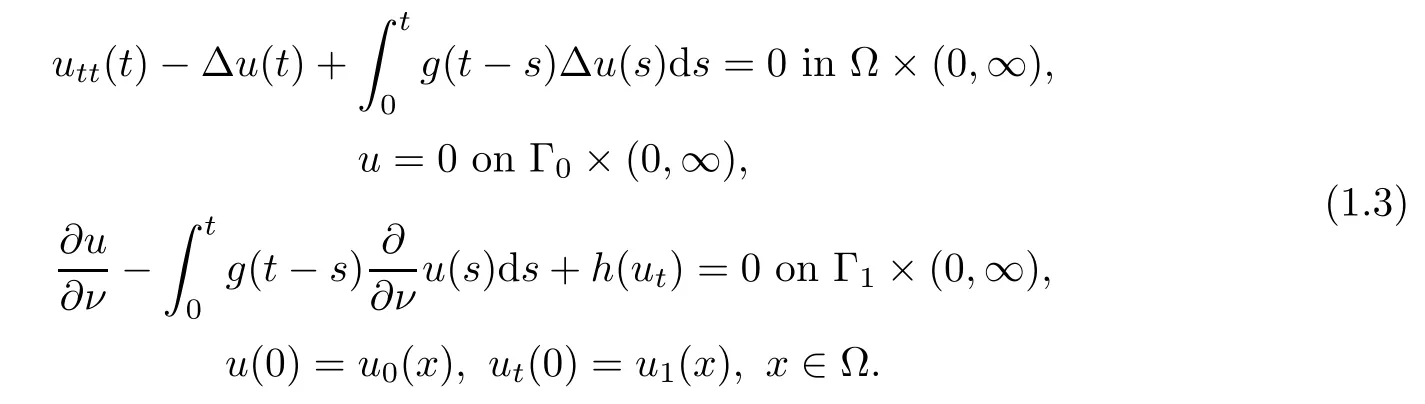
They showed the global existence of solutions and established some uniform decay results under quite restrictive assumptions on both the damping function h and the relaxation function g. Later,Cavalcanti et al.[6]generalized the result without imposing a growth condition on h and under a weaker assumption on g.Recently,Messaoudi and Mustafa[14]exploited some properties of convex functions[1]and the multiplier method to extend these results.They established an explicit and general decay rate result without imposing any restrictive growth assumption on damping term h and greatly weakened the assumption on g.
In the absence of Balakrishnan-Taylor damping(σ=0),equation(1.1)1is the model to describe the motion of deformable solids as hereditary effect is incorporated,which was first studied by Torrejon and Yong[18].They proved the existence of weakly asymptotic stable solution for large analytical datum.Later,Rivera[16]showed the existence of global solutions for small datum and the total energy decays to zero exponentially under some restrictions.
Conversely,in the presence of Balakrishnan-Taylor damping(σ/=0)and g=0,equation(1.1)1is used to study the flutter panel equation and to the spillover problem,which was initially proposed by Balakrishnan and Taylor in 1989[3],and Bass and Zes[4].The related problems also concerned by You[20],Clark[9],Tatar and Zarai[17,21]and Mu et al.[15].Recently,Zarai et al.[22]considered the following flutter equation with memory term:
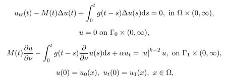
which arises in a wind tunnel experiment for a panel at supersonic speeds.They proved the global existence of solutions and a general decay result for the energy by using the multipliertechnique.
Motivated by previous works,we establish in this study the explicit and general decay rate for equations(1.1)under assumptions on g and h,without imposing a specific growth condition on the behavior of h near zero and greatly weakening the usual assumptions on relaxation function g.Our proof technique closely follows the arguments of[10,15,19],with some modifications being needed for our problem.The content of this paper is organized as follows.In Section 2,we provide assumptions that will be used later and state the local existence result Theorem 2.1.In Section 3,we prove our stability result that is given in Theorem 3.7.
2 Preliminary Results
In this section,we give assumptions and preliminaries that will be needed throughout the paper.First,we introduce the setwith the Hilbert structure induced by H1(?),we have thatis a Hilbert space.For simplicity,we denoteandAccording to(1.2),we have the imbedding:be the optimal constant of Sobolev imbedding which satisfies the inequality

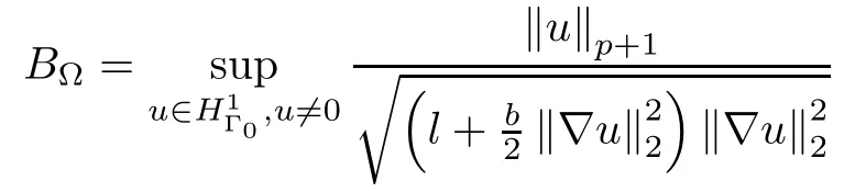
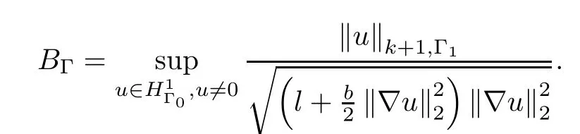
and we use the trace-Sobolev imbedding:In this case,the imbedding constant is denoted by B?,i.e.,

Next,we state the assumptions for problem(1.1).
(A1)g:[0,∞)→(0,∞)is a bounded C1function satisfying
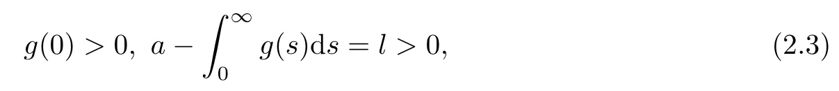
and there exists a non-increasing positive differentiable function ξ such thatfor all t≥0.

(A2) h:R→ R is a non-decreasing function with h(s)s≥0 for all s∈R and there exists a convex and increasing function H:R+→R+of class C1(R+)∩C2((0,∞))satisfying H(0)=0 and H is linear on[0,1]or H′(0)=0 and H′′>0 on(0,1]such that

where mqand Mqare positive constants.
Referring to[5,8,12,19],we state the local existence result without the proof.
Theorem 2.1 Let the initial data(u0,u1)∈H1Γ0×L2(?).Suppose that hypotheses(A1)-(A2)and(1.2)hold.Then there exists a weak solution u of problem(1.1)satisfying
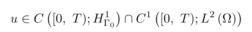
for some T>0.
3 Uniform Decay
In this section,we shall discuss the decay rate estimates for problem(1.1)providing that h satisfies(2.5)with q=1,that is,

The energy function associated with problem(1.1)is defined as

where
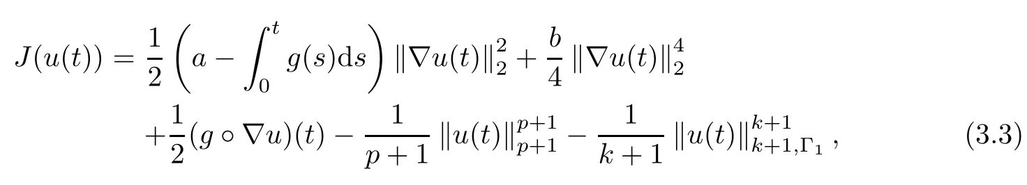
and

Adopting the proof of[13,14],we have the following result.
Lemma 3.1 Let u be the solution of problem(1.1),then,E(t)is a non-increasing function on[0,T)and

Next,we define a functional F introduced by Cavalcanti et al.[5],which helps in establishing desired results.Setting

where
and
Remark 3.2 (i)As in[5],we can verify that the functional F is increasing in(0,λ0),decreasing in(λ0,∞),and F has a maximum at λ0with the maximum value
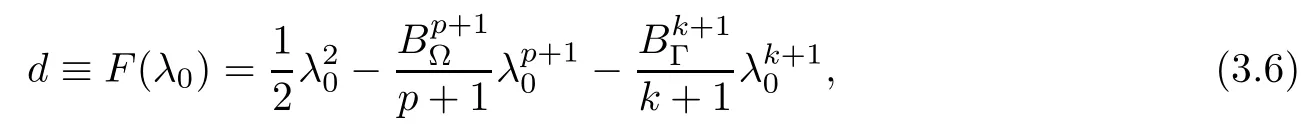
where λ0is the first positive zero of the derivative function F′(x).
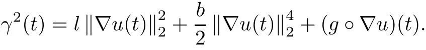
(ii)From(3.2),(3.3),(1.2),(2.3)and the definition of F,we have

where
Now,if one considers γ(t)<λ0,then,from(3.7),we get

which together with the identity

give


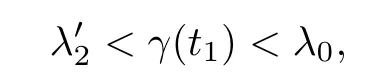
Proof Using(3.7)and considering E(t)is a non-increasing function,we obtainIn addition,from Remark 3.2(i),we see that F is increasing in(0,λ0),decreasing in(λ0,∞)and F(λ)→-∞as λ→∞.Thus,as E(0)<d,there exist λ′2<λ0<λ2such that F(λ′2)= F(λ2)=E(0).Besides,through the assumption γ(0)<λ0,we observe that


This implies that γ(0)≤λ′2.Next,we will prove that

To establish(3.12),we argue by contradiction.Suppose that(3.12)does not hold,then there exists t?∈(0,T)such that γ(t?)>λ′2.
Case 1 If λ′2<γ(t?)<λ0,then
This contradicts(3.11).
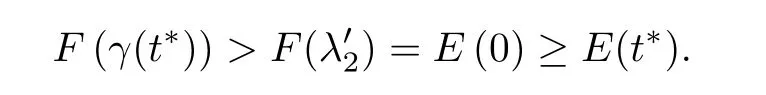
Case 2 If γ(t?)≥λ0,then by continuity of γ(t),there exists 0<t1<t?such that
then
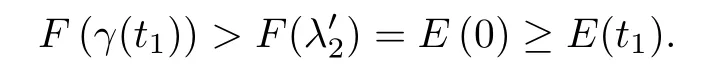
This is also a contradiction of(3.11).Thus,we have proved(3.10).
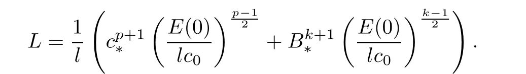
Proof It follows from(3.10),(3.9)and(3.7)that

Thus,we establish the boundedness of utin L2(?)and the boundedness of u inMoreover, from(2.1),(2.2)and(3.13),we also obtain
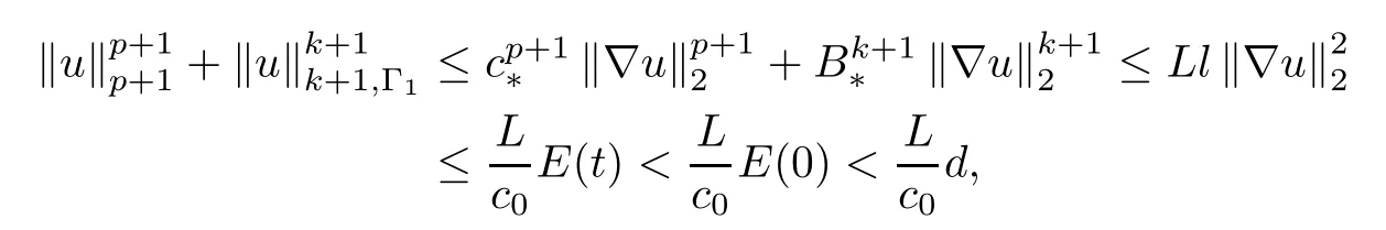
which implies that the boundedness of u in Lp+1(?)and in Lk+1(Γ1)withHence,it must have T=∞.
Now,we shall investigate the asymptotic behavior of the energy function E(t).First,we define some functionals and establish several lemmas.Let

where

and M,ε are some positive constants to be be specified later.
Lemma 3.5 There exist two positive constants β1and β2such that the relation

holds,for ε>0 small enough while M>0 is large enough.
Proof By H¨older's inequality,Young's inequality,(2.1)and(2.3),we deduce that
|G(t)-ME(t)|≤ε|Φ(t)|+|Ψ(t)|
whereEmploying(3.13)and selecting ε>0 small enough and M sufficiently large,there exist two positive constants β1and β2such that


Lemma 3.6 Let(A1)-(A2)and(1.2)hold.Assume thatλ0and E(0)<d.Furthermore,if E(0)is small enough,then,for any t0>0,the functional G(t)verifies,along solution of(1.1)and for t≥t0,

where αi,i=1-4 are some positive constants.
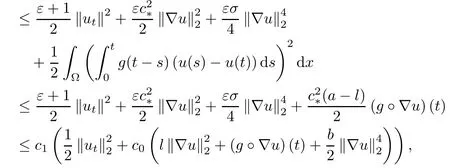
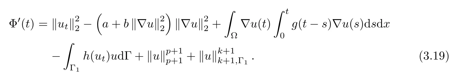
Proof In the following,we estimate the derivative of G(t).From(3.15)and(1.1),we have
Employing H¨older's inequality,Young's inequality,(2.3)and(2.2),the third and fourth terms on the right-hand side of(3.19)can be estimated as follows,for η,δ>0,

and

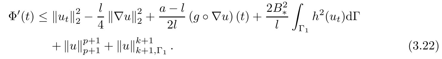
A substitution of(3.20)-(3.21)into(3.19)yields

Letting η=l2>0 andin above inequality,we obtain
Next,we estimate Ψ′(t).Taking the derivative of Ψ(t)in(3.16)and using(1.1),we obtain

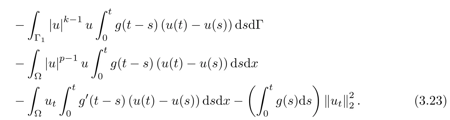
Similar to deriving(3.22),in what follows we will estimate the right-hand side of(3.23).Using Young's inequality,H¨older's inequalityby(3.4),and applying(2.3)and(2.2),we have,for δ>0,

and

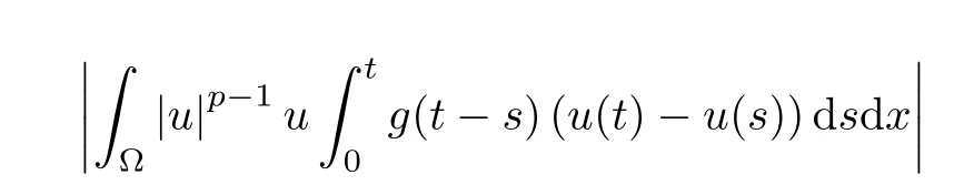
As for the the fifth and sixth terms on the right-hand side of(3.23),utilizing H¨older's inequality,Young's inequality,(2.1)-(2.3)and(3.13),we obtain

andExploiting H¨older's inequality,Young's inequality and(A1)to estimate the seventh term,we have
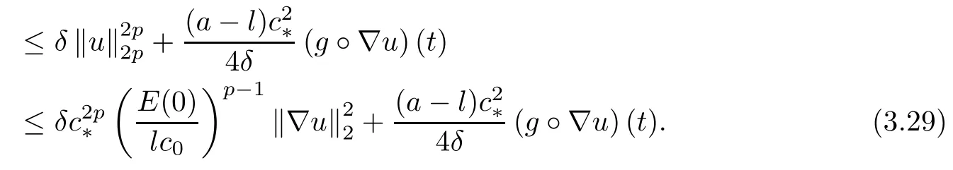

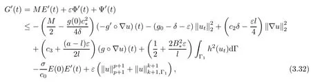
Then,combining these estimates(3.24)-(3.30),(3.23)becomes

where

and

Hence,we conclude from(3.14),(3.4),(3.22),and(3.31)that
where we have used the fact that for any t0>0,
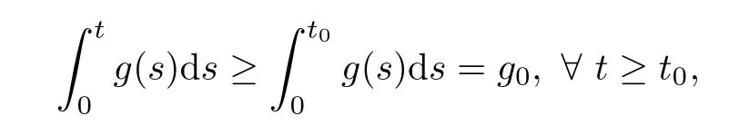
because g is positive and continuous with g(0)>0.At this point,we choose ε>0 small enough so that Lemma 3.5 holds andOnce ε is fixed,we choose δ to satisfy
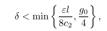
and then pick M sufficiently large such that.Thus,for all t≥t0,we arrive at
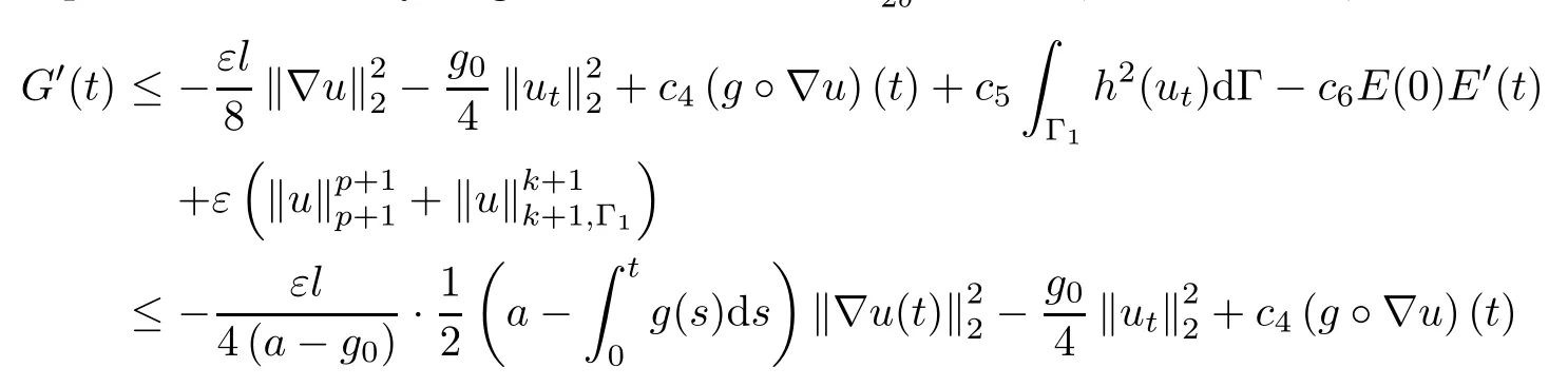

with some positive constants ci,i=4,5,6.Additionally,observing the fact thatdue toandand employing the definition of E(t)by(3.2)and usingby(3.13),we deduce that
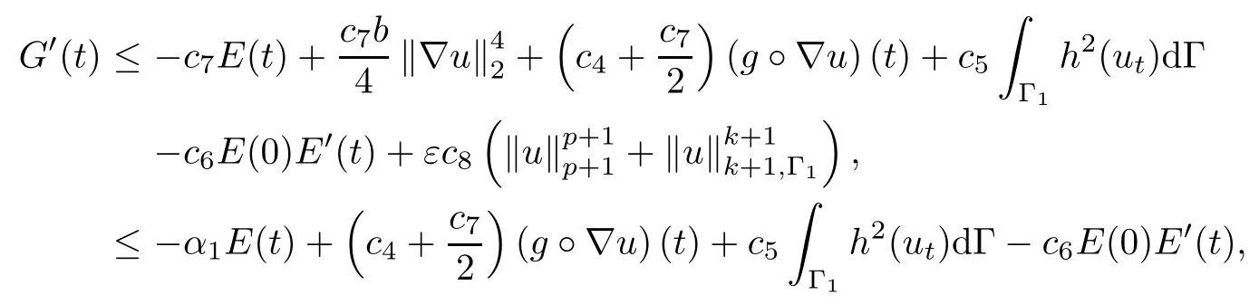
where

and

Hence,if E(0)is small enough,then not only the condition E(0)<d is satisfied,but also α1>0 is assured.Therefore,we have,for t≥t0,

where αj,j=1-4 are all positive constants.This completes the proof. □
Before stating our main result,we need to recall that if φ is a proper convex function from R to R∪{∞},then its convex conjugate φ?is defined as

Now,we are ready to prove our main results by adopting and modifying the arguments in[10,11,19].We consider the following partition of Γ1

Theorem 3.7 Let(A1)-(A2)and(1.2)hold.Assume thatγ(0)<λ0and E(0)<d.Furthermore,if E(0)is small enough,then,for each t0>0 and k1,k2and ε0are positive constants,the solution energy of(1.1)satisfies
where
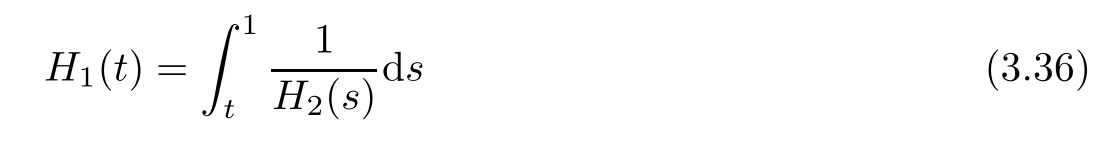
and
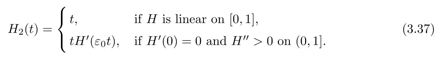
Proof The global existence of solution u of(1.1)is guaranteed directly by Theorem 3.4. Next,we consider the following two cases:(i)H is linear on[0,1]and(ii)H′(0)=0 and H′′>0 on(0,1].
Case 1 H is linear on[0,1].In this case,there exists α′1>0 such that|h(s)|≤α′1|s|,for all s∈R.By(3.4),we have
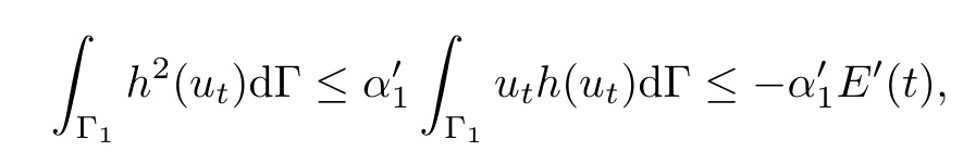
which together with(3.33)implies that

where H2(s)=s and c9=α′1α3+α4E(0).
Case 2 H′(0)=0 and H′′>0 on(0,1].In this case,we first estimateRΓ1h2(ut)dΓ on the right-hand side of(3.33).Given(3.1),noting that H-1is concave and increasing and using Jensen's inequality and(3.4),we deduce that
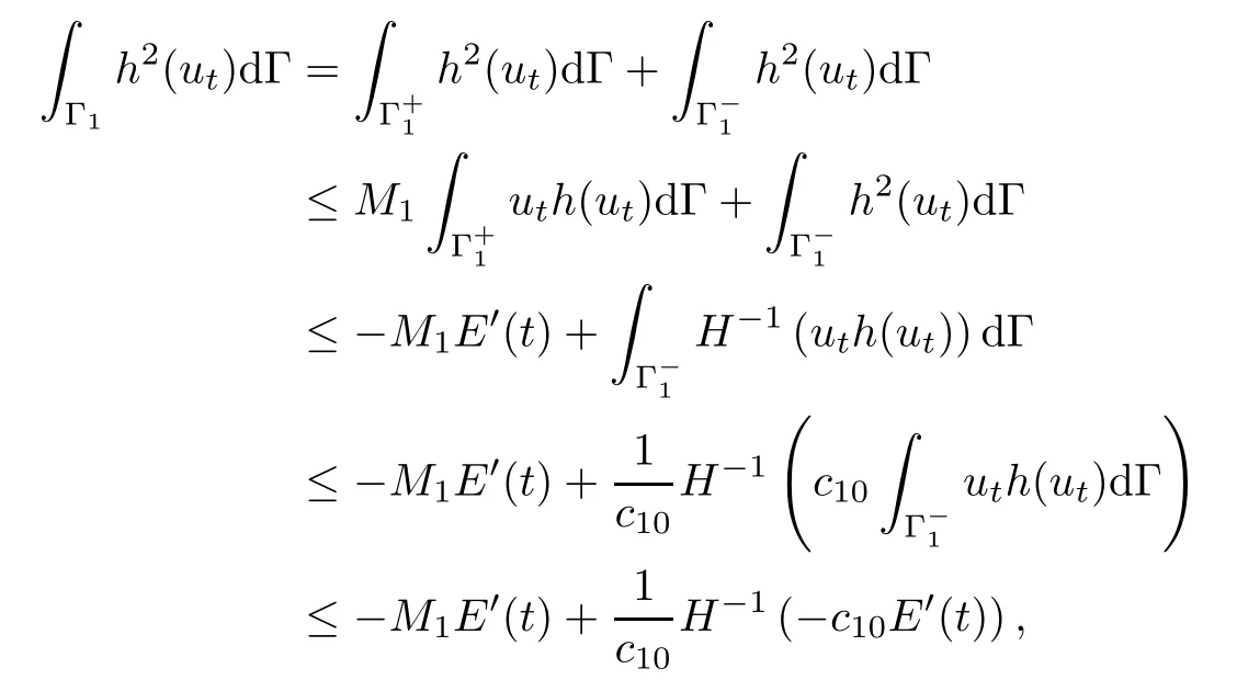

where


where ε0>0 and β>0 to be determined later.Then,using E′(t)≤0,H′′(t)≥0,and(3.39),we obtain
Let H?denote the Legendre transform of H defined by(3.34),then(see[2])

and H?satisfies the following inequalityFurther,using(3.43)and noting that H′(0)=0,(H′)-1is increasing and H is also increasing yield


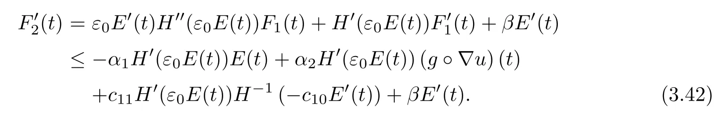
Taking H′(ε0E(t))=A and H-1(-c10E′(t))=B in(3.42),applying(3.45)and(3.44),and noting that 0≤H′(ε0E(t))≤H′(ε0E(0))due to H′is increasing,we obtain
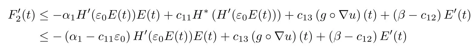
with c12=c10c11and c13=α2·H′(ε0E(0))>0.Thus,choosing 0<ε0<α1c11,β> c12and using E′(t)≤0 by(3.4),we have

where H2(s)=sH′(ε0s)and c14is a positive constant.
Let
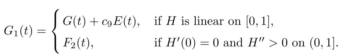
Then,by Lemma 3.5 and the definition of F2by(3.40)-(3.41),there exist β′1,β′2>0 such that

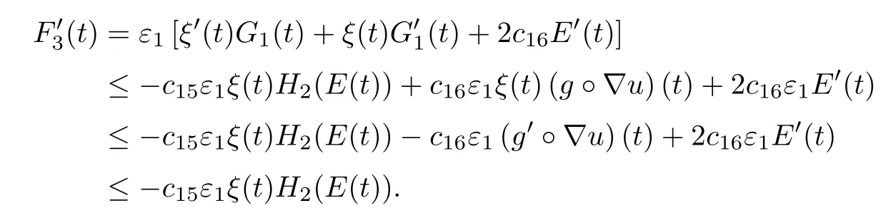
and from(3.38)and(3.46),we have

where c15and c16denote some positive constants.In addition,using(3.47)and ξ(t)≤ξ(0)by(A1),we see that

with l1=β′1ξ(0)+2c16>0.Now,we define

which is equivalent to E(t)by(3.47).Thanks to(3.48),(2.4)and(3.4),we arrive at
Exploiting the fact that H2is increasing,using(3.49)and noting 0<ε1<1l1by(3.50),we obtain
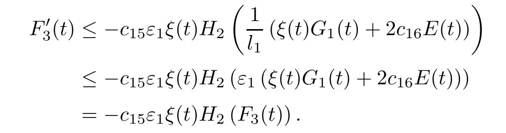
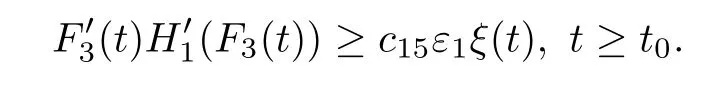
Integrating above inequality over(t0,t)and noting that H-11is decreasing on(0,1],we deduce that

where we require ε1>0 sufficiently small so that

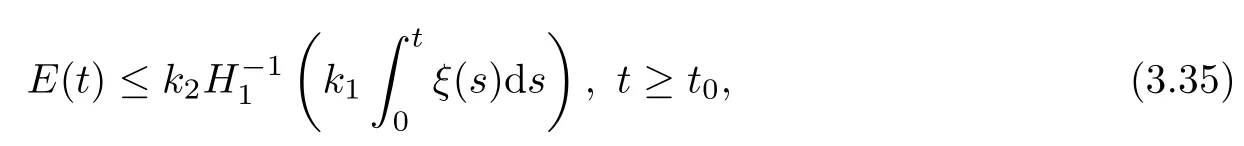
Consequently,the equivalent relation between of F3and E yields
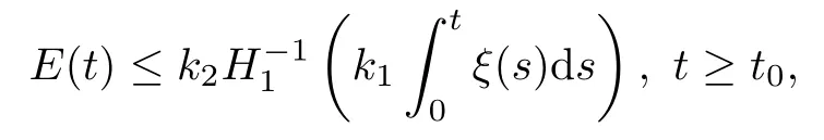
where k1and k2are positive constants.Hence,we complete the proof.
[1]Alabau-Boussouira F.On convexity and weighted integral inequalities for energy decay rates of nonlinear dissipative hyperbolic systems.Appl Math Optim,2005,51:61-105
[2]Arnold V L.Mathematical Methods of Classical Mechanics.New York:Springer-Verlag,1989
[3]Balakrishnan A V,Taylor L W.Distributed parameter nonlinear damping models for flight structures//Proceedings“Daming 89”,F(xiàn)light Dynamics Lab and Air Force Wright Aeronautical Labs.WPAFB,1989
[4]Bass R W,Zes D.Spillover nonlinearity,and flexible structures//Taylor L W,ed.The Fourth NASA Workshop on Computational Control of Flexible Aerospace Systems.NASA Conference Publication 10065,1991:1-14
[5]Cavalcanti M M,Cavalcanti V N D,Lasiecka I.Well-posedness and optimal decay rates for the wave equation with nonlinear boundary damping-source interaction.J Diff Eqns,2007,236:407-459
[6]Cavalcanti M M,Cavalcanti V N D,Martinez P.General decay rate estimates for viscoelastic dissipative systems.Nonlinear Anal,TMA,2008,68:177-193
[7]Cavalcanti M M,Cavalcanti V N D,F(xiàn)ilho J S Prates,Soriano J A.Existence and uniform decay rates for viscoelastic problems with nonlinear boundary damping.Differ Integral Equ,2001,14:85-116
[8]Cavalcanti M M,Cavalcanti V N D,Soriano J A.Global solvability and asymptotic stability for the wave equation with nonlinear feedback and source term on the boundary.Adv Math Sci Appl,2006,16:661-696
[9]Clark H R.Elastic membrane equation in bounded and unbounded domains.Electron J Qual Theory Differ Equ,2002,11:1-21
[10]Guessmia A,Messaoudi S A.General energy decay estimates of Timoshenko systems with frictional versus viscoelastic damping.Math Methods Appl Sci,2009,32:2102-2122
[11]Ha T G.On viscoelastic wave equation with nonlinear boundary damping and source term.Commun Pure Appl Anal,2010,6:1543-1576
[12]Lasiecka I,Tataru D.Uniform boundary stabilization of semilinear wave equations with nonlinear boundary damping.Differ Integral Equ,1993,6:507-533
[13]Messaoudi S A.General decay of solutions of a viscoelastic equation.J Math Anal Appl,2008,341:1457-1467
[14]Messaoudi S A,Mustafa M I.On convexity for energy decay rates of a viscoelastic equation with boundary feedback.Nonlinear Anal,TMA,2010,72:3602-3611
[15]Mu Chunlai,Ma Jie.On a system of nonlinear wave equations with Balakrishnan-Taylor damping.Z Angew Math Phys,2014,65(1):91-113
[16]Rivera J E M.Global solution on a quasilinear wave equation with memory.Bolletino UMI,1994,7B(8): 289-303
[17]Tatar N-e,Zarai A.Exponential stability and blow up for a problem with Balakrishnan-Taylor damping. Demonstr Math,2011,44(1):67-90
[18]Torrej′on R M,Young J.On a quasilinear wave equation with memory.Nonlinear Anal,TMA,1991,16: 61-78
[19]Wu S T.General decay and blow-up of solutions for a viscoelastic equation with a nonlinear boundary damping-source interactions.Z Angew Math Phys,2012,63:65-106
[20]You Y.Intertial manifolds and stabilization of nonlinear beam equations with Balakrishnan-Taylor damping. Abstr Appl Anal,1996,1:83-102
[21]Zarai A,Tatar N-e.Global existence and polynomial decay for a problem with Balakrishnan-Taylor damping.Arch Math(BRNO),2010,46:157-176
[22]Zarai A,Tatar N-e,Abdelmalek S.Elastic membrance equation with memory term and nonlinear boundary damping:global existence,decay and blowup of the solution.Acta Math Sci,2013,33B(1):84-106
?Received August 19,2014.
 Acta Mathematica Scientia(English Series)2015年5期
- Acta Mathematica Scientia(English Series)的其它文章
- ALL MEROMORPHIC SOLUTIONS OF AN AUXILIARY ORDINARY DIFFERENTIAL EQUATION AND ITS APPLICATIONS?
- APPROXIMATION OF COMMON FIXED POINT OF FAMILIES OF NONLINEAR MAPPINGS WITH APPLICATIONS?
- SOME COMPLETELY MONOTONIC FUNCTIONS ASSOCIATED WITH THE q-GAMMA AND THE q-POLYGAMMA FUNCTIONS?
- SUB-ADDITIVE PRESSURE ON A BOREL SET?
- AN APPLICABLE APPROXIMATION METHOD AND ITS APPLICATION?
- ORBITAL INSTABILITY OF STANDING WAVES FOR THE GENERALIZED 3D NONLOCAL NONLINEAR SCHR¨ODINGER EQUATIONS?